SpectraMax iD3s and iD5e overview
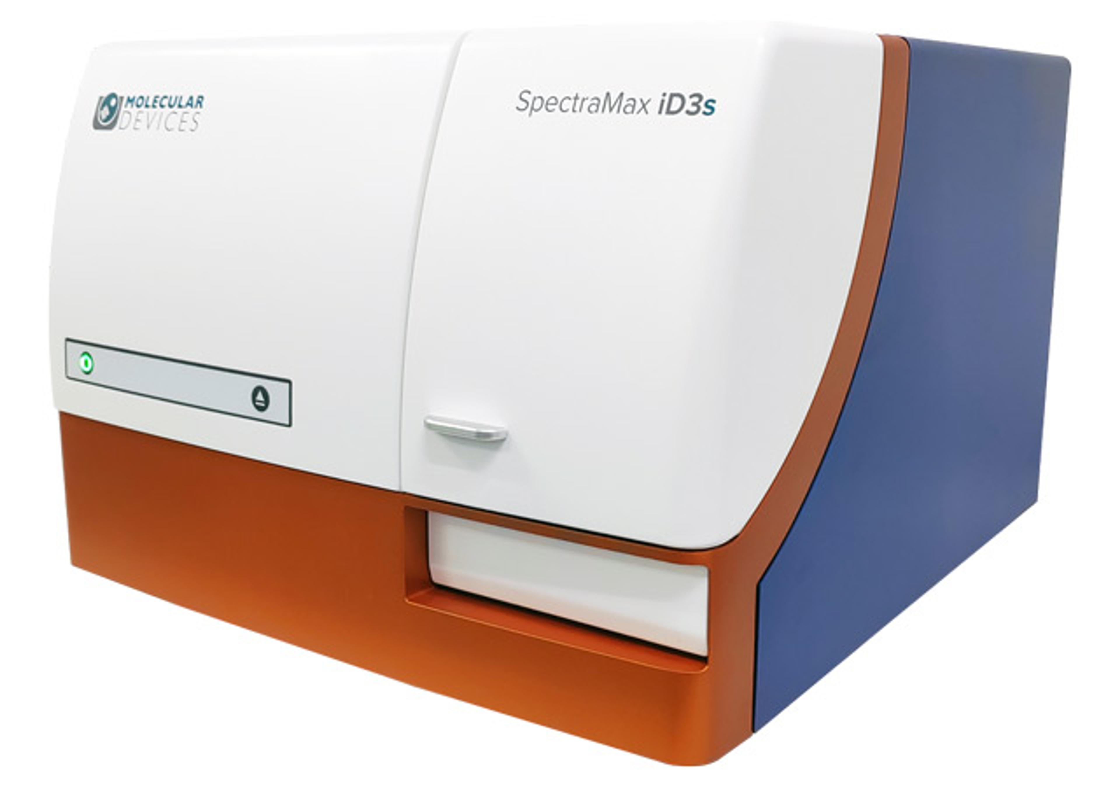
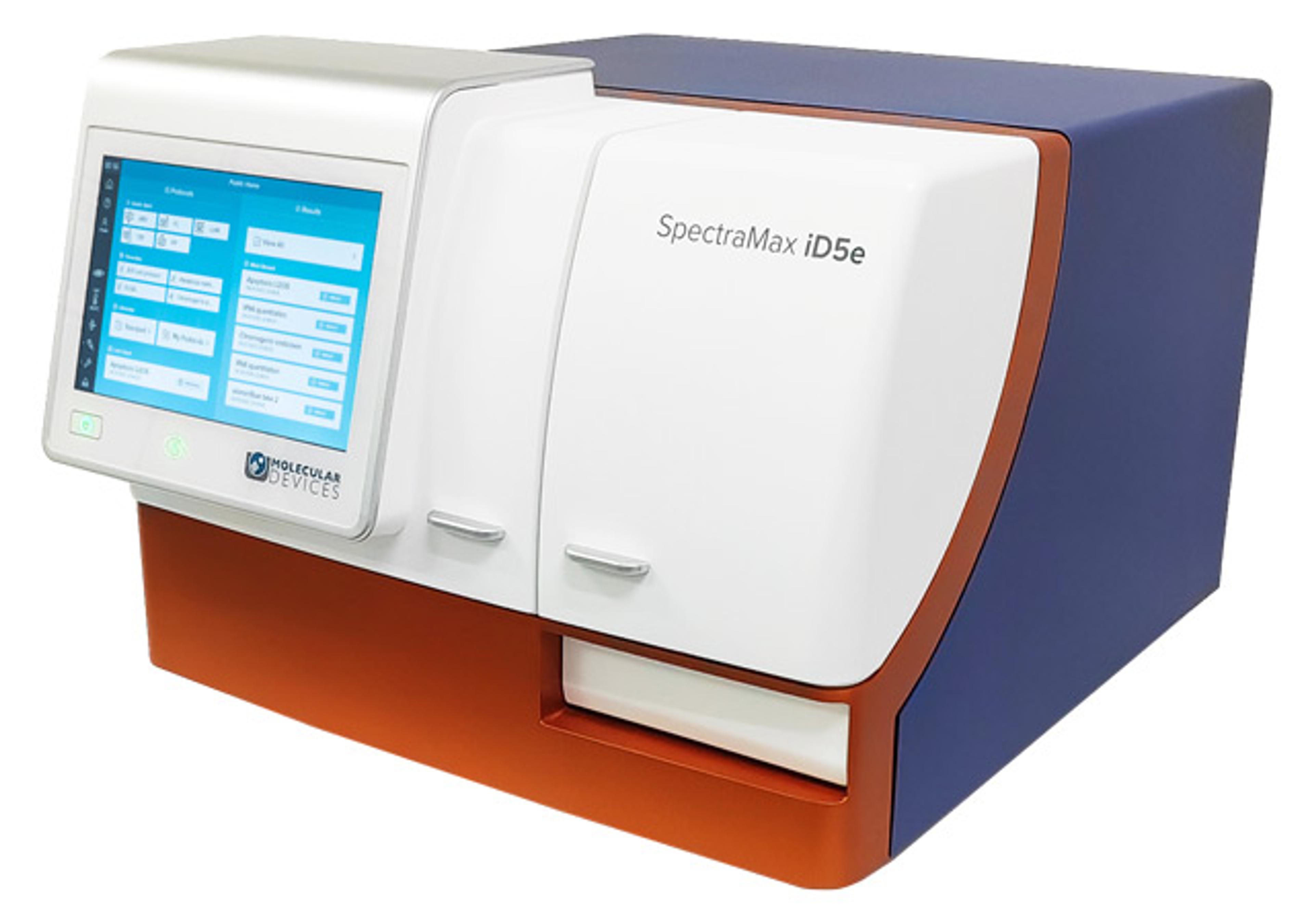
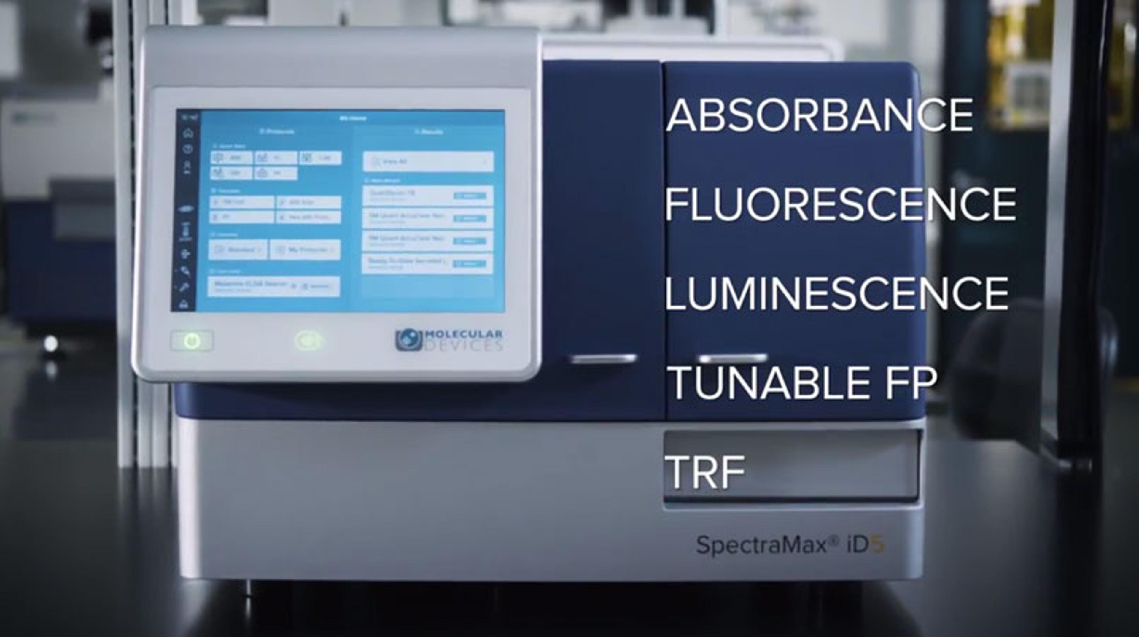
14 Sept 2026Explore the advanced capabilities of the Molecular Devices® SpectraMax® iD3s and iD5e microplate readers. These instruments offer versatile detection modes, including UV-Vis absorbance, fluorescence, and luminescence, with enhanced sensitivity through an ultra-cooled PMT. Discover features like hybrid optics, temperature control, and intelligent optimization tools within SoftMax Pro® software for comprehensive data analysis.
About the company

Molecular Devices®
Molecular Devices is one of the world’s leading providers of high-performance bioanalytical measurement systems, software and consumables for life science research, pharmaceutical and biotherapeutic development. Included within a broad product portfolio are platforms for high-throughput screening, genomic and cellular analysis, colony selection and microplate detection. These leading-edge products enable scientists to improve productivity and effectiveness, ultimately accelerating research and the discovery of new therapeutics. Molecular Devices is committed to the continual development of innovative solutions for life science applications. The company is headquartered in Silicon Valley, California, with offices around the globe. For more information, please visit www.moleculardevices.com.
General Inquiry - USA & Canada: +1 800-635-5577 General Inquiry - Europe: 00800 665 32860 Sales +1 877-589-2214 Support +1 800 635 5577
Video transcript
Show transcript
1
00:00:02.040 --> 00:00:05.190
Good morning and good afternoon to everybody, and welcome to today's
2
00:00:05.250 --> 00:00:10.905
webinar. My name is Michael Mendelson, and I'm a
3
00:00:10.950 --> 00:00:13.951
senior field application scientist in molecular devices.
4
00:00:15.316 --> 00:00:19.620
Today, we're going to be discussing the next generation of molecular devices plate
5
00:00:19.650 --> 00:00:23.970
readers, the SpectraMax ID3-S and ID5-E.
6
00:00:25.230 --> 00:00:31.020
These plate readers are an evolution of our ID series instruments, which have been
7
00:00:31.050 --> 00:00:34.231
positioned globally as one of our flagship readers.
8
00:00:37.231 --> 00:00:41.220
Today, we're going to be discussing the ID series instruments and their basic
9
00:00:41.250 --> 00:00:46.710
features. We'll also give you the brief differences between the ID3-S and the
10
00:00:46.800 --> 00:00:47.670
ID5-E.
11
00:00:49.350 --> 00:00:54.330
After going over the basic features of the ID series instruments, we are going to
12
00:00:54.420 --> 00:01:00.120
go into talking about what's new on the ID3-S and ID5-E.
13
00:01:00.180 --> 00:01:04.651
This is where we'll go over our new innovations to improve the ID series
14
00:01:04.711 --> 00:01:05.371
instruments.
15
00:01:07.080 --> 00:01:11.580
After that, we will go into SoftMax Pro and give you all a brief introduction on
16
00:01:11.610 --> 00:01:14.461
our industry-leading software, SoftMax Pro.
17
00:01:15.255 --> 00:01:20.250
This is a software that's able to do both acquisition and analysis all in one basic
18
00:01:20.340 --> 00:01:20.865
package.
19
00:01:22.321 --> 00:01:26.551
We will now move on in the webinar by providing you with an introduction to the ID
20
00:01:26.580 --> 00:01:29.821
series instruments, the ID3-S and the ID5-E.
21
00:01:30.870 --> 00:01:36.180
In this portion of the webinar, we will talk about what makes the ID3-S and ID5-E
22
00:01:36.359 --> 00:01:39.719
both unique and their shared features.
23
00:01:39.780 --> 00:01:44.220
To begin this discussion, we will start by talking about the ID3-S.
24
00:01:47.461 --> 00:01:52.336
The three in the name of the ID3-S stands for the read modes that it's able to read
25
00:01:52.380 --> 00:01:58.260
within. The ID3-S comes with three read modes, including UV-Vis
26
00:01:58.320 --> 00:02:02.400
absorbance with a spectral range of 230 to 1,000 nanometers.
27
00:02:03.420 --> 00:02:07.755
The ID3-S can also do top and bottom reading fluorescence, as well as
28
00:02:07.801 --> 00:02:11.310
luminescent-based applications.
29
00:02:11.340 --> 00:02:15.405
The ID3-S by design is a monochromator-based system.
30
00:02:16.485 --> 00:02:21.930
Monochromators provide you with wavelength tunability within all of the read modes,
31
00:02:21.960 --> 00:02:25.275
where you can tune your wavelength within one nanometer increments.
32
00:02:26.641 --> 00:02:32.175
Within each of the three read modes on the ID3-S, there are four read types.
33
00:02:33.421 --> 00:02:37.410
An endpoint read will take the point of detection at the center of the well at a
34
00:02:37.470 --> 00:02:43.125
single time point. This will include applications like your BCA assays for
35
00:02:43.141 --> 00:02:47.415
protein quantitation or your DNA quant applications.
36
00:02:49.035 --> 00:02:53.715
The kinetic read type will allow you to take multiple reads across a defined
37
00:02:54.150 --> 00:02:54.735
runtime.
38
00:02:56.745 --> 00:03:01.830
The well scan read type is very beneficial for any assays with adherent cells at
39
00:03:01.860 --> 00:03:02.805
the bottom of the well.
40
00:03:04.050 --> 00:03:08.490
Well scan allows you to take multiple points of detection across the area of the
41
00:03:08.520 --> 00:03:14.340
well. And the last read type is spectrum scanning, which allows you to
42
00:03:14.460 --> 00:03:20.041
scan across the spectral range within each of the three read modes.
43
00:03:20.101 --> 00:03:25.515
The ID3-S also has the ability to be upgraded with a dual injector module that has
44
00:03:25.531 --> 00:03:30.345
an ultra-low dead volume. We will talk about this more in later slides.
45
00:03:31.664 --> 00:03:37.590
The ID3-S also comes with SoftMax Pro, which provides it with ease of use
46
00:03:37.620 --> 00:03:41.265
and a package that provides data acquisition and analysis.
47
00:03:46.710 --> 00:03:52.140
The ID5-E is going to come with a few extra read modes that we call our
48
00:03:52.201 --> 00:03:57.585
advanced read modes, bringing it up to five total read modes able to read within
49
00:03:57.630 --> 00:03:58.380
the instrument.
50
00:03:59.744 --> 00:04:04.921
The ID5-E will come with the same three read modes the ID3-S has with absorbance,
51
00:04:05.010 --> 00:04:10.140
fluorescence, and luminescence, but the ID5-E will also have the ability to do
52
00:04:10.201 --> 00:04:15.601
advanced read modes such as time resolve fluorescence, fluorescence polarization,
53
00:04:15.630 --> 00:04:18.585
and fluorescence resonance energy transfer or FRET.
54
00:04:19.740 --> 00:04:25.664
To do these assays, the ID5-E employs a filter set to provide you with
55
00:04:25.710 --> 00:04:29.100
the increased sensitivity required for these advanced read modes.
56
00:04:30.600 --> 00:04:36.494
Just like the ID3-S, the ID5-E also has the upgradable option of a
57
00:04:36.510 --> 00:04:37.695
dual injector module.
58
00:04:39.420 --> 00:04:44.341
Using our ScanLater Western Blot detection technology, you are also able to read
59
00:04:44.400 --> 00:04:46.500
Western Blots on the ID5-E.
60
00:04:48.781 --> 00:04:53.940
The biggest difference between the ID5-E and the ID3-S is that the
61
00:04:54.091 --> 00:04:57.150
ID5-E is a hybrid optical system.
62
00:04:58.350 --> 00:05:04.005
It still has the tunability and flexibility provided by the monochromators,
63
00:05:04.560 --> 00:05:10.440
but the ID5-E can also include six excitation or six emission
64
00:05:10.531 --> 00:05:11.820
filters in the unit.
65
00:05:13.560 --> 00:05:17.670
This provides you with the ability to increase your sensitivity for assays which
66
00:05:17.730 --> 00:05:22.531
you are developing and also provide you with a wider dynamic range.
67
00:05:24.841 --> 00:05:30.540
And the ID5-E is also going to have similar features to the ID3-S, such
68
00:05:30.600 --> 00:05:35.400
as the ultra-cooled PMT and our auto PMT features, which we will discuss in later
69
00:05:35.490 --> 00:05:35.940
slides.
70
00:05:43.920 --> 00:05:49.260
Both ID series instruments come equipped with a high-efficiency four-monochromator
71
00:05:49.275 --> 00:05:54.330
design. This provides you with two monochromators on the excitation side of your
72
00:05:54.360 --> 00:05:58.244
light path and two monochromators on the emission side of your light path,
73
00:05:59.040 --> 00:06:04.350
providing you with more wavelength tunability while also conserving the photons
74
00:06:04.440 --> 00:06:08.970
needed for your assay and removing any background light from entering your light
75
00:06:09.031 --> 00:06:09.390
path.
76
00:06:11.880 --> 00:06:15.975
Both instruments also use a xenon flash lamp as their light source.
77
00:06:16.815 --> 00:06:21.750
The xenon flash lamp in the instrument only powers on when it's being used during
78
00:06:21.781 --> 00:06:26.220
an assay, so it's reliable to over a billion flashes with easy
79
00:06:26.250 --> 00:06:32.070
validation. One of the most important features on the ID series instruments is the
80
00:06:32.130 --> 00:06:37.350
ultra-cooled PMT. We will talk a little bit more about the ultra-cooled PMT in
81
00:06:37.410 --> 00:06:42.855
later slides. This is a patented technology meant to reduce background noise from
82
00:06:42.901 --> 00:06:48.780
your sample, providing you with a more sensitive signal and a wider dynamic range.
83
00:06:52.500 --> 00:06:57.270
The biggest functional difference between the ID3-S and the
84
00:06:57.360 --> 00:07:02.460
ID5-E is that the ID5-E has a hybrid optical system.
85
00:07:02.475 --> 00:07:08.115
This means that the ID5-E can use either monochromators or filters or a combination
86
00:07:08.160 --> 00:07:11.326
of the two to get the best results for every assay.
87
00:07:12.151 --> 00:07:16.454
Having flexibility between your wavelength selection really gives you the ability
88
00:07:16.454 --> 00:07:21.630
to optimize your assays and perform assay development at your own speed for the
89
00:07:21.720 --> 00:07:27.660
best sensitivity. The ID5-E can accommodate six filters on the excitation
90
00:07:27.780 --> 00:07:30.975
slider and six filters on the emission slider.
91
00:07:31.770 --> 00:07:36.045
Filters are easily swapped out and read automatically within the instrument and
92
00:07:36.091 --> 00:07:40.350
input into the software, where you can access them through the dropdown menu.
93
00:07:41.250 --> 00:07:46.395
We have a list of many filters for all different fluorophores and read modes and
94
00:07:46.410 --> 00:07:49.920
are able to custom build filters if that's what's required.
95
00:07:54.480 --> 00:07:59.640
This slide displays some features that are on both of the instruments.
96
00:08:00.690 --> 00:08:06.510
Both the ID5-E and the ID3-S can accommodate temperatures with temperature
97
00:08:06.540 --> 00:08:09.390
control up to 65 degrees Celsius.
98
00:08:11.010 --> 00:08:15.151
Both of the instruments in their standard configuration have three modes of
99
00:08:15.240 --> 00:08:20.716
shaking: linear, which would shake the plate side to side, orbital, which would
100
00:08:20.790 --> 00:08:26.040
shake the plate in an orbital or circular fashion, and double orbital, which would
101
00:08:26.100 --> 00:08:30.451
shake the plate in a figure eight or an infinity sign fashion.
102
00:08:31.951 --> 00:08:37.095
One of the newer features on the instruments is the option to have advanced shaking
103
00:08:37.230 --> 00:08:40.681
specific for microbial growth applications.
104
00:08:40.711 --> 00:08:45.181
We will discuss this in further detail when we talk about the new features on the
105
00:08:45.240 --> 00:08:50.686
ID series instruments. Both the ID5-E and the ID3-S can
106
00:08:50.730 --> 00:08:56.490
accommodate plate types down to six wells and all the way up to 384-well
107
00:08:56.520 --> 00:09:02.370
plates, and everything in between, including 12, 24, 48, and
108
00:09:02.610 --> 00:09:08.595
96-well plates. Both instruments have the option to add an optional
109
00:09:08.640 --> 00:09:13.170
cuvette adapter if cuvette research is something that you're interested in.
110
00:09:14.496 --> 00:09:20.346
Our cuvette adapter can accommodate three working cuvettes as well as one blank.
111
00:09:22.476 --> 00:09:28.386
And again, we cannot stress how important the patented ultra-cooled PMT is
112
00:09:28.416 --> 00:09:32.466
for better background noise reduction for a more sensitive signal in fluorescence
113
00:09:32.496 --> 00:09:37.356
and luminescence. We will go in a little bit more detail on the principles and the
114
00:09:37.416 --> 00:09:40.566
function of the ultra-cooled PMT in the next slide.
115
00:09:44.286 --> 00:09:47.811
You've heard me mention it a few times, but now I want to go in a little bit more
116
00:09:47.826 --> 00:09:52.956
detail on one of our unique patented features, the ultra-cooled PMT.
117
00:09:53.826 --> 00:09:58.491
If you're not familiar with what the acronym PMT stands for, it stands for
118
00:09:58.507 --> 00:10:03.846
photomultiplier tube. This is your platform of detection for any fluorescence or
119
00:10:03.906 --> 00:10:06.666
luminescent-based applications.
120
00:10:06.696 --> 00:10:10.851
When an instrument is operating, you can imagine that it's going to produce some
121
00:10:10.866 --> 00:10:16.027
residual heat within the system. A standard PMT will take that heat,
122
00:10:16.507 --> 00:10:22.266
convert it into signal, contributing to background noise in your sample.
123
00:10:22.296 --> 00:10:27.936
What we do on our ultra-cooled PMT is we cool the PMT down to negative five degrees
124
00:10:27.966 --> 00:10:33.936
Celsius, thereby removing any heat contribution from the signal, which will provide
125
00:10:33.996 --> 00:10:39.246
you with a wider dynamic range, lower background, and a better lower limit of
126
00:10:39.306 --> 00:10:45.186
detection. This can sometimes be the difference between a false negative
127
00:10:45.201 --> 00:10:49.326
and actually reading signal on your plate reader.
128
00:10:49.341 --> 00:10:53.676
The ultra-cooled PMT will provide you with more accurate distinction between weak
129
00:10:53.766 --> 00:10:58.611
signal and no signal, and can be the difference between an assay working and not
130
00:10:58.626 --> 00:11:04.146
working. If you look at the graph to the right, we will display this graphically.
131
00:11:05.496 --> 00:11:10.507
The grayer bar on the graph displays your dynamic range with a standard PMT,
132
00:11:11.046 --> 00:11:16.116
whereas the lighter shaded graph is going to show you your dynamic range with a
133
00:11:16.176 --> 00:11:17.196
cooled PMT.
134
00:11:18.576 --> 00:11:23.286
Another way that I like to explain this is if you're looking at a mountain and the
135
00:11:23.376 --> 00:11:28.716
top of the mountain is covered with clouds, that is what your system is like with a
136
00:11:28.806 --> 00:11:34.027
non-cooled PMT. With a cooled PMT, when you look at the mountain,
137
00:11:34.596 --> 00:11:39.426
there's no more clouds covering the peak, and now you can resolve the smallest
138
00:11:39.486 --> 00:11:43.086
portion on the visible eye of the mountain, which is the peak of the mountain.
139
00:11:44.616 --> 00:11:50.257
The ultra-cooled PMT will be on both of the instruments, the iD3s and the
140
00:11:50.346 --> 00:11:51.246
iD5e.
141
00:11:55.806 --> 00:11:59.856
The next patented feature that's going to be available on both instruments is our
142
00:11:59.946 --> 00:12:01.341
auto PMT feature.
143
00:12:02.976 --> 00:12:08.286
Auto PMT allows you to read assays with an extremely wide dynamic range.
144
00:12:09.396 --> 00:12:15.246
What the auto PMT does is it automatically adjusts the PMT gain according to signal
145
00:12:15.277 --> 00:12:21.081
intensity, reading each well at the highest PMT gain, where if any of those wells
146
00:12:21.126 --> 00:12:26.331
saturate, it will read them again under the medium PMT gain, and if any of those
147
00:12:26.346 --> 00:12:30.785
wells saturate, it'll read it under the low PMT gain.
148
00:12:30.936 --> 00:12:36.486
After this, it will automatically normalize your data based on the lowest PMT gain
149
00:12:36.576 --> 00:12:42.277
used, providing you with a dynamic range that extends up to seven logs.
150
00:12:42.336 --> 00:12:46.836
What you can see to the right is the settings in SoftMax Pro, where you have the
151
00:12:46.926 --> 00:12:52.146
fixed settings of high, medium, and low, and at the top, you have the automatic PMT
152
00:12:52.206 --> 00:12:52.911
gain setting.
153
00:12:54.216 --> 00:13:00.007
The graph to the left shows you the reads at the three different fixed PMT gain
154
00:13:00.066 --> 00:13:05.616
settings, where the high is in green, the medium is in blue, and the low is in
155
00:13:05.646 --> 00:13:11.436
purple. What you can see from this graph is that in the high PMT gain read, you
156
00:13:11.466 --> 00:13:14.826
have a lot of saturation at the higher end of your curve.
157
00:13:16.026 --> 00:13:20.646
When you read under medium, you're able to resolve a few more points on the curve,
158
00:13:20.767 --> 00:13:23.947
but you're still saturating at the top end of your curve.
159
00:13:25.056 --> 00:13:30.576
When you read it again at the low PMT gain, you're able to resolve the full curve,
160
00:13:31.056 --> 00:13:36.186
but you see that you start to lose linearity at the lower end of the curve.
161
00:13:37.386 --> 00:13:42.276
What we do to combat this is the auto PMT normalization, where we now normalize
162
00:13:42.336 --> 00:13:47.496
based off of the three points so that now you maintain linearity across the whole
163
00:13:47.511 --> 00:13:50.136
entire dynamic range of the assay.
164
00:13:52.416 --> 00:13:57.291
Just to conclude, this auto PMT feature is a very powerful feature if you have
165
00:13:57.396 --> 00:14:02.496
very, very bright and very, very dim samples on the same plate, where now you're
166
00:14:02.556 --> 00:14:05.947
able to maintain linearity across that dynamic range.
167
00:14:12.876 --> 00:14:17.257
With the use of SoftMax Pro, both instruments will also come with a few
168
00:14:17.407 --> 00:14:20.586
optimization features to help you in your research.
169
00:14:21.727 --> 00:14:26.390
The first optimization feature is going to be microplate optimization.
170
00:14:26.436 --> 00:14:31.416
The second optimization feature is going to be read height adjustment, adjusting
171
00:14:31.447 --> 00:14:33.936
the Z-axis of the PMT.
172
00:14:35.436 --> 00:14:40.356
And the last is going to be wavelength optimization, or our Spectral Optimization
173
00:14:40.386 --> 00:14:46.026
Wizard. We will go in a bit more detail in each of these three optimization
174
00:14:46.056 --> 00:14:48.007
features in the next few slides.
175
00:14:49.267 --> 00:14:52.686
To do that, we're going to start with the Spectral Optimization Wizard.
176
00:14:57.816 --> 00:15:03.456
The Spectral Optimization Wizard is an optimization feature that comes with
177
00:15:03.486 --> 00:15:07.176
SoftMax Pro that is available within the fluorescence read
178
00:15:07.206 --> 00:15:13.056
mode. The Spectral Optimization Wizard requires you
179
00:15:13.116 --> 00:15:19.041
to have a well with whatever your sample fluorophore is, as well as a well with
180
00:15:19.056 --> 00:15:21.352
whatever your blank or your buffer is.
181
00:15:22.566 --> 00:15:26.856
The Spectral Optimization Wizard will then perform a spectrum scan on both the
182
00:15:26.947 --> 00:15:32.556
excitation and emission wavelength pair for both of those wells.
183
00:15:32.616 --> 00:15:37.146
Once it's completed with that scan, it will provide you with the optimal excitation
184
00:15:37.176 --> 00:15:42.636
and emission wavelength pair for that fluorophore, given the signal-to-noise ratio
185
00:15:42.665 --> 00:15:44.586
between the fluorophore and the buffer.
186
00:15:45.575 --> 00:15:49.852
It will produce for you a graph such as you see on the screen here, where you can
187
00:15:49.896 --> 00:15:54.322
move the hairpin trigger to the most red spot, which would tell you what the best
188
00:15:54.366 --> 00:15:58.477
working wavelength set is for that fluorophore.
189
00:15:58.536 --> 00:16:03.216
This will also allow you to see any secondary peaks that you might have missed to
190
00:16:03.276 --> 00:16:08.346
show you how you can optimize your wavelength for that fluorophore even further.
191
00:16:13.176 --> 00:16:17.241
The next two optimization features that we'll discuss are both available through
192
00:16:17.257 --> 00:16:21.096
SoftMax Pro and are pre-read optimization options.
193
00:16:22.447 --> 00:16:27.636
Option one is microplate optimization, requiring you to have sample in the four
194
00:16:27.786 --> 00:16:33.186
corner wells of your microplate. This optimization wizard will then scan those four
195
00:16:33.216 --> 00:16:38.736
corner wells and spit out the optimal dimensions for the microplate and
196
00:16:38.826 --> 00:16:41.241
automatically input them into the software.
197
00:16:42.396 --> 00:16:47.916
You will also be able to visualize and choose the exact center of the well using a
198
00:16:47.977 --> 00:16:52.611
hairpin trigger to more accurately read your data and ensure that you're reading
199
00:16:52.626 --> 00:16:57.157
from the center of the well for that specific plate type.
200
00:16:57.201 --> 00:17:02.106
The Microplate Optimization Wizard is especially beneficial for six to 48 or
201
00:17:02.286 --> 00:17:06.322
384-well plates, where the dimensions vary from vendor to vendor.
202
00:17:07.326 --> 00:17:12.187
It can also be very beneficial if you're running 96-well half-area plates.
203
00:17:13.687 --> 00:17:18.336
This optimization wizard prevents you from having to surf the internet to find the
204
00:17:18.366 --> 00:17:22.566
specific dimensions for a lot and manually input them into the software.
205
00:17:25.056 --> 00:17:28.986
The next optimization feature we'll discuss is the read height adjustment
206
00:17:29.136 --> 00:17:34.191
optimization feature. This is going to be available in any of the read modes that
207
00:17:34.236 --> 00:17:40.116
use a PMT. The Read Height Adjustment Wizard requires you to have
208
00:17:40.176 --> 00:17:45.666
wells with your sample in them, where the optimization wizard will then optimize
209
00:17:45.726 --> 00:17:48.006
the height of the detector above the well.
210
00:17:49.626 --> 00:17:54.096
This optimization wizard is sensitive to volumetric changes.
211
00:17:54.156 --> 00:17:58.536
So if you ran the optimization wizard for one specific assay and then either
212
00:17:58.566 --> 00:18:03.036
reduced or increased the sample volume, you will need to run this optimization
213
00:18:03.096 --> 00:18:03.786
wizard again.
214
00:18:10.116 --> 00:18:16.086
The next shared feature between both instruments is the ability to add on a dual
215
00:18:16.146 --> 00:18:20.016
injector system at any point in which you have the instrument
216
00:18:22.038 --> 00:18:27.198
The dual injector module is housed in the right side of the instrument, as shown in
217
00:18:27.228 --> 00:18:28.339
the images to the right.
218
00:18:29.598 --> 00:18:34.008
It's a peristaltic pump that can move both forward and reverse.
219
00:18:35.089 --> 00:18:39.603
The dual injectors are enabled for all read modes and have a few unique features
220
00:18:39.649 --> 00:18:45.423
associated with them. One feature is overflow detection, where there's a sensor at
221
00:18:45.438 --> 00:18:49.818
the tip of the injector, where if a liquid or a fluid touches the tip of the
222
00:18:49.878 --> 00:18:55.368
injector, it will stop the assay from progressing to avoid overflowing the well and
223
00:18:55.399 --> 00:18:57.738
damaging the instrument and the assay.
224
00:18:59.388 --> 00:19:03.813
You also have a feature called Smart Inject, which will shake the plate while
225
00:19:03.828 --> 00:19:08.568
you're injecting into the well to ensure homogenous distribution of your substrate
226
00:19:08.628 --> 00:19:14.268
or your reagent. The dual injectors can dispense in volumes as low as one
227
00:19:14.298 --> 00:19:19.578
microliter and as high as the maximal allowable volume of your plate type, and
228
00:19:19.608 --> 00:19:22.098
within one microliter increments in between.
229
00:19:23.988 --> 00:19:29.628
It has a low dead volume of 10 microliters, and it achieves this by having the
230
00:19:29.688 --> 00:19:35.298
reverse peristaltic flow, returning any unused reagent back to its
231
00:19:35.418 --> 00:19:38.627
tubing infrastructure at the conclusion of the assay.
232
00:19:40.068 --> 00:19:44.418
The injectors are also going to dispense at a speed of 100 microliters per second
233
00:19:44.899 --> 00:19:49.518
and come with great tutorials for washing, priming, calibration, and tube
234
00:19:49.578 --> 00:19:55.038
replacement that will be available either on the touchscreen of the ID5e or within
235
00:19:55.098 --> 00:19:57.468
SoftMax Pro for the ID3S.
236
00:19:59.058 --> 00:20:04.038
These injectors are specifically tailored for flash luminescence assays such as
237
00:20:04.128 --> 00:20:05.748
dual luciferase reactions.
238
00:20:12.168 --> 00:20:17.688
We'll now move on to discuss new features that come on the ID Series instruments,
239
00:20:17.748 --> 00:20:22.518
which include an advanced shaking component and environmental control.
240
00:20:23.598 --> 00:20:27.018
We'll start by discussing the advanced shaking option.
241
00:20:27.198 --> 00:20:31.878
Both of these features are available on both of the instruments.
242
00:20:35.718 --> 00:20:40.248
The advanced shaking option is a feature that came to our plate readers through
243
00:20:40.278 --> 00:20:45.198
customer feedback from those wanting a more robust system for their microbial
244
00:20:45.318 --> 00:20:46.233
growth assays.
245
00:20:47.583 --> 00:20:53.358
The advanced shaking option will improve the robustness of the shaft that holds
246
00:20:53.388 --> 00:20:56.028
and shakes the plate within the plate reader.
247
00:20:56.808 --> 00:21:01.159
It also allows you to be a little bit more specific in terms of your speed,
248
00:21:01.458 --> 00:21:05.028
diameter, and shake mode within the instrument.
249
00:21:06.964 --> 00:21:12.363
This advanced shaking option is meant to maximize your microbial growth assays by
250
00:21:12.409 --> 00:21:14.418
enhancing the robustness of the reader.
251
00:21:15.738 --> 00:21:20.388
This is specifically for people who are doing continuous growth assays with
252
00:21:20.448 --> 00:21:26.089
continuous shaking over long periods of time, such as 24, 48, or 72
253
00:21:26.178 --> 00:21:26.598
hours.
254
00:21:28.218 --> 00:21:33.183
The shake option with advanced shaking allows you to adjust the shake diameter, has
255
00:21:33.198 --> 00:21:38.553
a configurable RPM speed, which is dependent on plate type, shake diameter, and
256
00:21:38.568 --> 00:21:44.298
shake mode, and allows you to be more specific in the total shaking cycle to
257
00:21:44.388 --> 00:21:45.888
better meet customer needs.
258
00:21:47.628 --> 00:21:51.933
When you have the advanced shaking option, you also still have the standard shake
259
00:21:52.038 --> 00:21:57.572
option. To initiate the advanced shake option, all you need to do is check a box
260
00:21:57.618 --> 00:21:58.847
within SoftMax Pro.
261
00:22:02.418 --> 00:22:08.223
The next new feature that comes on the ID Series units is the ability
262
00:22:08.328 --> 00:22:11.268
to have environmental control within your plate chamber.
263
00:22:12.918 --> 00:22:18.618
This is enabled by the SpectraMax AER or air exchange regulator, used as the
264
00:22:18.678 --> 00:22:24.138
gas mixer on the system. This should provide you with a walkaway solution for
265
00:22:24.198 --> 00:22:29.103
long-term lifestyle assays that maximize your lab performance.
266
00:22:30.438 --> 00:22:36.168
This is going to be compatible with both the ID3S and ID5e and can be
267
00:22:36.288 --> 00:22:38.358
added to the instrument at any time.
268
00:22:41.839 --> 00:22:46.863
The control of oxygen and CO2 is going to be software-driven, allowing you to
269
00:22:46.968 --> 00:22:52.788
change your oxygen within the plate chamber from ambient down
270
00:22:52.818 --> 00:22:58.788
to 1% within 0.1% increments, and the CO2
271
00:22:58.818 --> 00:23:04.278
from ambient to 15%, again in 0.1% increments.
272
00:23:08.268 --> 00:23:14.238
These values are traceable in the software and allow you to put
273
00:23:14.298 --> 00:23:19.038
them into the audit trail if you're in a GxP or compliant environment.
274
00:23:28.368 --> 00:23:33.018
In this slide, we just wanted to show you what the SoftMax Pro control interface
275
00:23:33.078 --> 00:23:35.628
looks like for environmental control.
276
00:23:37.159 --> 00:23:41.778
You will have in your instrument settings the ability to see what the set point is
277
00:23:41.839 --> 00:23:44.718
for your CO2 and O2 settings.
278
00:23:45.978 --> 00:23:51.318
When you click the gas control button, it will open up a window that allows you to
279
00:23:51.333 --> 00:23:56.748
turn the environmental control or the gas control on and dictate the
280
00:23:56.778 --> 00:24:02.058
percentage of either CO2, O2, or both that you want in the plate chamber.
281
00:24:04.368 --> 00:24:09.318
You're also able to use the gas control feature within our workflow editor to do
282
00:24:09.378 --> 00:24:13.278
more advanced protocol development within SoftMax Pro.
283
00:24:16.668 --> 00:24:22.518
You will also notice that in the settings information, it
284
00:24:22.548 --> 00:24:27.078
will give you the set points to the right with the rest of your acquisition
285
00:24:27.168 --> 00:24:28.938
settings for that specific assay.
286
00:24:38.238 --> 00:24:42.152
We'll use this slide to show you some data collected using the environmental
287
00:24:42.228 --> 00:24:47.899
control for three-day live-cell assays using U2OS cells.
288
00:24:48.888 --> 00:24:52.998
What this graph below is showing you that the performance of the environmental
289
00:24:53.072 --> 00:24:58.188
control is very similar to that of the incubator.
290
00:24:58.203 --> 00:25:03.243
The experimental info for this was the plate was using an IB seal to help with
291
00:25:03.258 --> 00:25:08.464
humidity control, where the plate reader was set at 37 degrees and CO2 set at
292
00:25:08.748 --> 00:25:10.998
5% in the SpectraMax AER.
293
00:25:12.468 --> 00:25:16.728
What you can see is the blue and the red are going to be the incubator and the
294
00:25:16.758 --> 00:25:21.918
environmental control, whereas the green is the use of no environmental control at
295
00:25:22.128 --> 00:25:27.183
all. The conclusion from this assay is that ATP levels measured with
296
00:25:27.228 --> 00:25:32.688
CellTiter-Glo demonstrate comparable levels for the incubator and the
297
00:25:32.808 --> 00:25:36.063
ID gas mixer, the ID Series gas mixer.
298
00:25:39.468 --> 00:25:43.548
The next piece of data we wanted to show you is just to show you successful
299
00:25:43.563 --> 00:25:49.488
real-time viability monitoring using the RealTime-Glo assay kit.
300
00:25:49.548 --> 00:25:54.978
What you're seeing here is cells plated at three different densities and tracked
301
00:25:55.038 --> 00:26:00.738
over 72 hours. This was done in the SpectraMax ID
302
00:26:00.798 --> 00:26:06.258
Series with an AER gas mixer to avoid the need of transferring the plate to an
303
00:26:06.318 --> 00:26:07.968
incubator after each read.
304
00:26:09.603 --> 00:26:14.508
This data shows successful viability assessment or successful growth across the
305
00:26:14.748 --> 00:26:16.788
72-hour period.
306
00:26:20.419 --> 00:26:26.178
We'll now move our conversation forward by talking about SoftMax Pro.
307
00:26:27.169 --> 00:26:31.758
SoftMax Pro is an industry-leading software that has both data acquisition and
308
00:26:31.818 --> 00:26:36.948
analysis all in one easy-to-use and refined package.
309
00:26:41.298 --> 00:26:46.833
When you purchase an ID3S or an ID5e, you will receive four perpetual
310
00:26:46.938 --> 00:26:52.608
licenses that you can apply to a PC to control the instrument with
311
00:26:52.639 --> 00:26:53.538
SoftMax Pro.
312
00:26:55.339 --> 00:26:59.508
What you're looking at now is the general interface for SoftMax Pro.
313
00:26:59.538 --> 00:27:04.968
Built within the Windows operating system and user interface, this SoftMax Pro
314
00:27:04.998 --> 00:27:10.024
interface is very easy to use with many one-click or one-touch
315
00:27:10.158 --> 00:27:11.149
accessibilities.
316
00:27:12.798 --> 00:27:17.058
Some benefits that we provide to our customers in SoftMax Pro include the protocol
317
00:27:17.178 --> 00:27:17.613
manager.
318
00:27:18.858 --> 00:27:24.198
The protocol manager has a protocol library of over 200 pre-populated protocols.
319
00:27:25.687 --> 00:27:29.961
These protocols are there to help you when you're ready to run an assay on our
320
00:27:29.976 --> 00:27:34.927
plate readers. You can use these protocols as a scaffolding or a foundation to
321
00:27:34.957 --> 00:27:39.096
build your own working protocols for future use.
322
00:27:39.156 --> 00:27:42.877
All of these protocols are going to be available to you upon installation of
323
00:27:42.906 --> 00:27:43.866
SoftMax Pro.
324
00:27:50.616 --> 00:27:55.056
One of the big benefits to SoftMax Pro is the fact that you can do data acquisition
325
00:27:55.086 --> 00:27:58.146
and analysis all within one easy workflow.
326
00:27:59.302 --> 00:28:05.062
What I want to show you now is how we can take an already created protocol and get
327
00:28:05.106 --> 00:28:09.067
to analyze data using that protocol.
328
00:28:09.127 --> 00:28:13.446
To do that, I'm going to open a protocol from my own personal protocol library.
329
00:28:15.817 --> 00:28:20.346
What you can see here is a template already applied to the protocol, having the
330
00:28:20.437 --> 00:28:23.946
different groups in different colors and duplicate columns.
331
00:28:25.386 --> 00:28:30.336
You can also see that we have our data layout already set in tables to give us some
332
00:28:30.366 --> 00:28:31.971
important pieces of information,
333
00:28:33.396 --> 00:28:36.846
and we have a standard curve that is waiting to be plotted.
334
00:28:38.076 --> 00:28:42.606
What I'm going to do is just copy and paste this data here as I'm in a simulated
335
00:28:42.696 --> 00:28:43.326
interface.
336
00:28:45.321 --> 00:28:49.446
And now you'll see that once we've collected the data, our tables will be filled.
337
00:28:49.896 --> 00:28:52.596
We'll have a lot of analyzed data and information.
338
00:28:53.976 --> 00:28:57.666
And when we go to our curve, you'll see that the curve is already plotted with a
339
00:28:57.726 --> 00:29:01.927
fit applied to all four of the graphs.
340
00:29:05.046 --> 00:29:10.236
That is to show you one easy way of using SoftMax Pro, by having a pre-written or
341
00:29:10.266 --> 00:29:15.067
pre-canned protocol, so that when you're ready, all you need to do is press play to
342
00:29:15.096 --> 00:29:18.996
collect data and have already analyzed data once the read is completed.
343
00:29:21.471 --> 00:29:25.281
The next thing that we'd like to show you within SoftMax Pro is how you can take
344
00:29:25.326 --> 00:29:30.502
collected raw data and easily get to an analyzed data set in just a few clicks and
345
00:29:30.516 --> 00:29:35.766
a few minutes. To do this, we'll access some pre-collected data.
346
00:29:35.796 --> 00:29:41.391
You're seeing two wavelengths collected here, one at 450 nanometers and one at 630
347
00:29:41.466 --> 00:29:46.356
nanometers. One of the things I can do to this data is subtract the two wavelengths
348
00:29:46.416 --> 00:29:48.156
with each other using the Reduction tab.
349
00:29:48.966 --> 00:29:52.506
This is where you can perform mathematical calculations to your raw data within the
350
00:29:52.536 --> 00:29:53.002
software.
351
00:29:54.846 --> 00:29:58.177
I'm going to go ahead and subtract the wavelengths from each other and then choose
352
00:29:58.236 --> 00:30:03.906
the Display tab to display my reduced value in bold below my raw
353
00:30:04.386 --> 00:30:05.002
wavelengths.
354
00:30:06.457 --> 00:30:09.427
You're also able to view your data in a color map
355
00:30:11.586 --> 00:30:14.406
and with the reduced number below the color map.
356
00:30:16.656 --> 00:30:22.401
Beyond data visualization, to plot into these tables and into the graph, you need
357
00:30:22.416 --> 00:30:24.636
to apply a template within SoftMax Pro.
358
00:30:25.927 --> 00:30:30.156
So to do this, we'll take our standards and quickly plot a standard curve.
359
00:30:32.976 --> 00:30:34.567
We'll go ahead and quickly plot our
360
00:30:34.627 --> 00:30:39.306
unknowns.
361
00:30:42.966 --> 00:30:44.976
And we'll quickly plot a plate blank.
362
00:30:47.556 --> 00:30:51.036
When you look at this and see what I'm doing, I just would like you guys to know
363
00:30:51.067 --> 00:30:55.506
that this is something that you'll be trained on how to do upon purchase of the
364
00:30:55.567 --> 00:30:59.976
reader. Once I click OK, you'll notice that my data changes a little bit to
365
00:31:00.006 --> 00:31:03.726
represent the background subtraction from our plate blank.
366
00:31:06.457 --> 00:31:10.086
When we scroll through the generated tables, you'll notice that there's a column
367
00:31:10.146 --> 00:31:13.446
for back calculation that has empty wells associated with it.
368
00:31:14.136 --> 00:31:18.846
To populate data in this column, we will need to apply a statistical fit to our
369
00:31:18.906 --> 00:31:23.226
standard curve. So let's go ahead and jump down to the standard curve and see what
370
00:31:23.286 --> 00:31:23.916
we observe.
371
00:31:25.177 --> 00:31:28.656
What you're seeing here is our data points plotted along the standard curve.
372
00:31:29.556 --> 00:31:35.136
If I want to apply a statistical fit, I can apply one of 22 different statistical
373
00:31:35.286 --> 00:31:37.416
fits into the data set.
374
00:31:43.177 --> 00:31:47.121
Once you apply your fit, if you scroll down, you'll get the logistical equation as
375
00:31:47.136 --> 00:31:51.516
well as the parameters that fit into the equation, your R squared, and in the case
376
00:31:51.576 --> 00:31:55.326
of a four-parameter logistic, the IC or EC50.
377
00:31:56.796 --> 00:32:01.716
These graphs are exportable. You can also save them, and you can add
378
00:32:01.806 --> 00:32:06.486
annotation as either text, image, or shape onto the graph.
379
00:32:07.986 --> 00:32:12.096
Another cool feature is you can right-click a data point and highlight the source
380
00:32:12.156 --> 00:32:13.596
for where that data is coming from.
381
00:32:14.196 --> 00:32:20.016
This is very beneficial to outlining or identifying why an error bar
382
00:32:20.106 --> 00:32:22.011
might be larger than the others.
383
00:32:24.636 --> 00:32:27.427
When we scroll through the tables now, you'll notice that the tables are fully
384
00:32:27.457 --> 00:32:28.161
populated
385
00:32:29.677 --> 00:32:33.546
and that now we have data that we can look at and observe.
386
00:32:37.536 --> 00:32:42.246
There is so much more to learn below the surface of SoftMax Pro, giving you the
387
00:32:42.336 --> 00:32:48.036
option to do many different forms of statistical or data analysis and customize how
388
00:32:48.096 --> 00:32:50.556
your data is output once you've collected it.
389
00:32:56.586 --> 00:32:59.556
That concludes the content portion of today's webinar.
390
00:33:00.786 --> 00:33:05.496
On this slide, you will see my name, title, and information, as well as information
391
00:33:05.556 --> 00:33:07.761
from Molecular Devices and our support team.
392
00:33:09.006 --> 00:33:13.041
Feel free to reach out should you have any questions or require any additional
393
00:33:13.086 --> 00:33:15.531
information about what we discussed today.