ELISA and advanced detection technologies

1
00:00:02.401 --> 00:00:06.660
Good morning everyone, and welcome to this webinar, ELISA and Beyond.

2
00:00:07.380 --> 00:00:10.860
My name is Teresa, and I'm here today with my colleague, Rebecca.

3
00:00:11.700 --> 00:00:17.130
Together, we will provide you some information about ELISA and other immunoassays.

4
00:00:18.030 --> 00:00:20.625
First of all, we will introduce ourselves.

5
00:00:23.940 --> 00:00:28.576
Hi again, my name is Teresa, and I'm working as a bioresearch field application

6
00:00:28.651 --> 00:00:34.425
scientist since January of 2021. Previously to joining the company, I did my

7
00:00:34.470 --> 00:00:37.770
PhD about nutrition and type 2 diabetes.

8
00:00:39.690 --> 00:00:41.731
What do I normally do on my free time?

9
00:00:42.540 --> 00:00:47.445
Well, I love to try new food, so consider myself as a foodie, and I also love

10
00:00:47.520 --> 00:00:52.995
reading books. In addition to that, I enjoy traveling, doing yoga, and I have

11
00:00:53.011 --> 00:00:57.901
started dancing. Now, I will pass on my colleague, Rebecca.

12
00:01:03.000 --> 00:01:05.340
Thank you, Teresa. Good morning everyone.

13
00:01:05.371 --> 00:01:10.410
My name is Rebecca, and I'm a field application scientist for Molecular Devices.

14
00:01:10.470 --> 00:01:15.270
My background is in neuroscience, where I studied in University College, Dublin.

15
00:01:15.360 --> 00:01:19.530
I joined Molecular Devices about a year ago and currently cover Ireland and the

16
00:01:19.560 --> 00:01:24.390
Nordics. Some of my hobbies include eating, as you can see here on the left,

17
00:01:25.321 --> 00:01:29.670
also running and tennis in my spare time, and I'm an avid animal lover.

18
00:01:29.700 --> 00:01:33.540
Here's a picture of my little dog, Willow, on the right.

19
00:01:33.690 --> 00:01:38.551
So to start off, here is a brief look at what we will cover today.

20
00:01:38.641 --> 00:01:44.010
We'll look at what is an ELISA, its three base detection modes, and then finally

21
00:01:44.070 --> 00:01:49.500
moving on to some more advanced technology such as HTRF and Alpha

22
00:01:49.530 --> 00:01:50.220
technology.

23
00:01:52.980 --> 00:01:54.930
So first off, what is an ELISA?

24
00:01:56.521 --> 00:02:01.410
ELISAs are a type of immunoassay that are commonly used to quantify levels of a

25
00:02:01.440 --> 00:02:03.211
specific target within a sample.

26
00:02:04.590 --> 00:02:10.230
Samples include serum, plasma, saliva, which you'll be familiar with the COVID

27
00:02:10.260 --> 00:02:14.760
tests, and also with pregnancy tests, as the example here is urine.

28
00:02:16.500 --> 00:02:21.300
There are four main types of ELISAs. The first one here is a direct ELISA.

29
00:02:22.560 --> 00:02:27.059
An antigen or sample is immobilized directly on the plate, and a conjugated

30
00:02:27.120 --> 00:02:30.120
detection antibody binds to the target protein.

31
00:02:31.500 --> 00:02:36.976
The substrate is then added in suspension, producing a signal that is directly

32
00:02:37.020 --> 00:02:40.110
proportional to the amount of analyte in the sample.

33
00:02:42.720 --> 00:02:48.510
These are used when assessing antibody affinity and specificity, and also when you

34
00:02:48.540 --> 00:02:51.540
want to investigate blocking or inhibitory interactions.

35
00:02:54.090 --> 00:02:59.101
An indirect ELISA is similar to a direct ELISA in that an antigen is immobilized

36
00:02:59.160 --> 00:03:04.935
again on a plate. But it includes a conjugated secondary antibody, shown here in

37
00:03:04.980 --> 00:03:09.585
blue, directed against the host species of the primary antibody, shown here in

38
00:03:09.720 --> 00:03:10.110
green.

39
00:03:11.610 --> 00:03:17.041
The suspended substrate then again produces a signal directly proportional to the

40
00:03:17.101 --> 00:03:17.970
amount of analyte

41
00:03:19.470 --> 00:03:20.970
or antigen bound in the well.

42
00:03:22.680 --> 00:03:25.560
So these are used when measuring endogenous antibodies.

43
00:03:27.510 --> 00:03:30.945
Moving on to a sandwich ELISA, which is the most common type of ELISA.

44
00:03:32.400 --> 00:03:38.310
Two specific antibodies are used to sandwich the antigen, commonly referred to

45
00:03:38.430 --> 00:03:44.085
as matched antibody pairs. A substrate then in suspension again is added

46
00:03:44.400 --> 00:03:48.480
and produces a signal that is directly proportional to the amount of antigen

47
00:03:48.510 --> 00:03:49.560
present in the sample.

48
00:03:50.851 --> 00:03:55.080
These are usually used when determining analyte concentration in a biological

49
00:03:55.230 --> 00:03:55.619
sample.

50
00:03:57.840 --> 00:04:02.160
And lastly, we have the competitive ELISAs, which are commonly used for small

51
00:04:02.190 --> 00:04:08.070
molecules when the protein of interest is too small to efficiently sandwich

52
00:04:08.101 --> 00:04:13.860
with two antibodies. So here the antigen competes with the reference antigen for

53
00:04:13.890 --> 00:04:17.430
binding of a specific amount of labeled antibody.

54
00:04:17.490 --> 00:04:22.574
The reference is pre-coded on a multi-well plate, and the sample is

55
00:04:22.620 --> 00:04:26.685
pre-incubated with the labeled antibody and added then to the wells.

56
00:04:28.170 --> 00:04:33.750
So depending on the amount of antigen in the sample, more or less free antibodies

57
00:04:33.781 --> 00:04:35.250
will be available to bind to the

58
00:04:35.310 --> 00:04:46.951
reference

59
00:04:47.010 --> 00:04:47.490
antigen.

60
00:04:48.990 --> 00:04:54.810
This means that the more antigen there is in the sample, the less reference

61
00:04:54.900 --> 00:04:58.230
antigen will be detected and the weaker the

62
00:04:58.290 --> 00:05:03.195
signal. These are usually used when determining

63
00:05:03.240 --> 00:05:06.930
concentrations of small molecules or hormones.

64
00:05:09.510 --> 00:05:15.345
So here is a table showing which ELISA to choose from and their advantages and

65
00:05:15.360 --> 00:05:16.230
disadvantages.

66
00:05:17.505 --> 00:05:20.220
For direct ELISAs, they're fast and simple.

67
00:05:21.031 --> 00:05:26.985
However, they can be less specific as it only uses one antibody and

68
00:05:27.000 --> 00:05:31.605
has potential for high background if all proteins from the sample are immobilized

69
00:05:31.650 --> 00:05:36.841
in the well. For indirect, amplification arises

70
00:05:37.440 --> 00:05:40.080
using the secondary antibody.

71
00:05:41.880 --> 00:05:46.410
There is, however, potential for cross-reactivity caused by the secondary antibody.

72
00:05:48.000 --> 00:05:53.730
For a sandwich ELISA, has the highest specificity and compatible with

73
00:05:53.880 --> 00:05:59.281
small matrices. However, the protocols can be long and challenging to develop.

74
00:06:00.570 --> 00:06:02.580
For a competitive ELISA,

75
00:06:04.170 --> 00:06:07.680
they have the ability to quantitate small molecules.

76
00:06:07.740 --> 00:06:12.525
However, again, they can be less specific since you're only using one antibody and

77
00:06:12.540 --> 00:06:18.525
requires the conjugate antigen. The illustration above shows

78
00:06:18.540 --> 00:06:20.790
a workflow for a typical sandwich ELISA.

79
00:06:22.470 --> 00:06:24.420
You can see here that there is eight steps.

80
00:06:26.550 --> 00:06:32.369
You have your 96 to 3L microplates where your antibody binds to the well,

81
00:06:33.451 --> 00:06:37.770
then the addition of your sample. And then here shown in red, you have your two

82
00:06:37.800 --> 00:06:43.740
washing steps, which can be very time consuming as it can take over an hour for

83
00:06:43.800 --> 00:06:49.620
these washing procedures. You usually wash the microplate three times in

84
00:06:49.680 --> 00:06:53.370
each wash steps, which can be a total of six washes.

85
00:06:55.140 --> 00:06:56.610
Then here with seven and eight,

86
00:06:57.870 --> 00:07:02.640
the microplate reader is used to detect the color change produced when the target

87
00:07:02.701 --> 00:07:07.890
antigen is present. And then lastly, you have your software, which is used to plot

88
00:07:07.951 --> 00:07:11.640
your standard curves and calculate results.

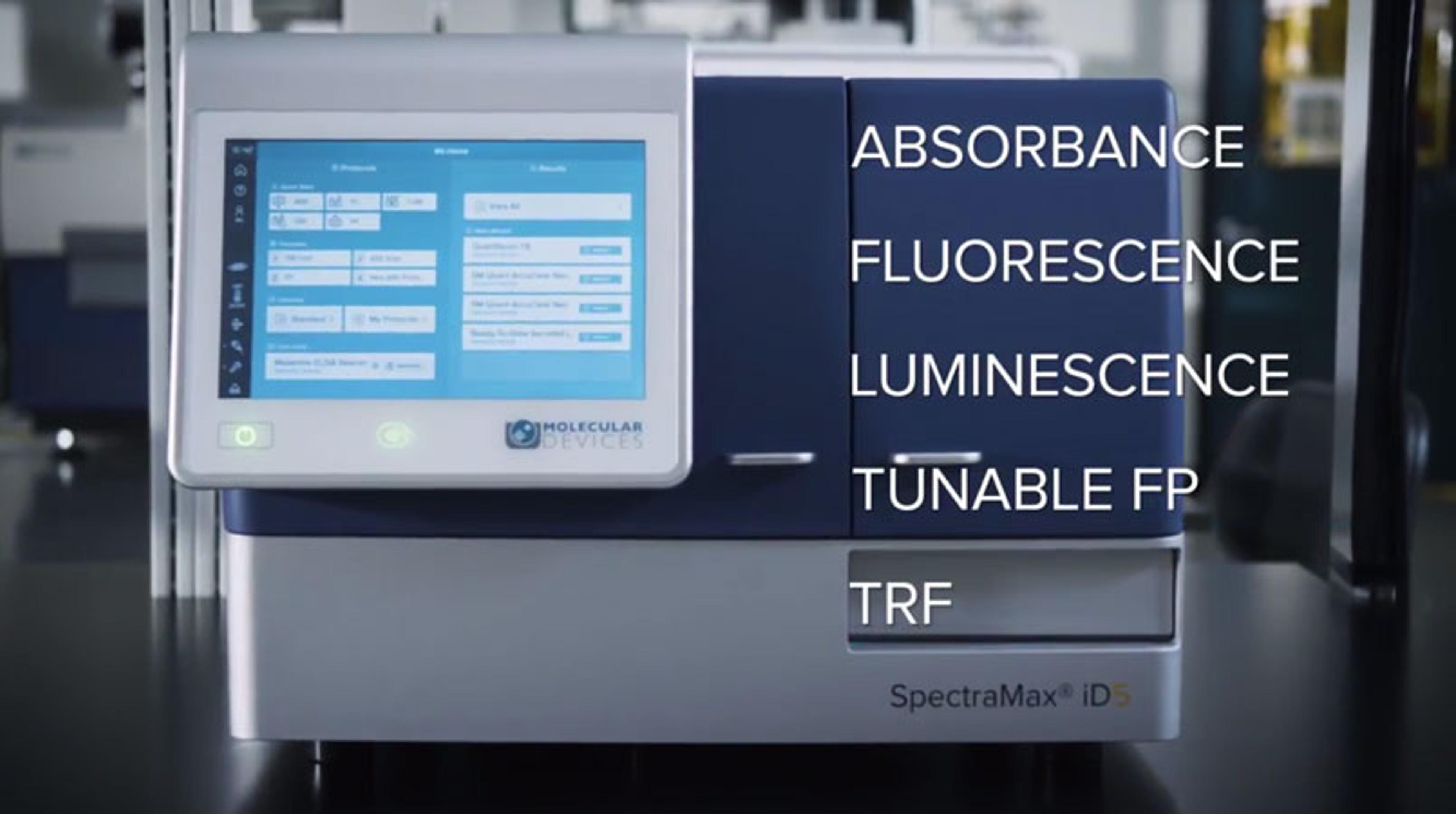
89
00:07:11.655 --> 00:07:14.160
This workflow can also be fully automated.

90
00:07:16.320 --> 00:07:20.460
We all know too well that manual microplate washing with pipettes can be very

91
00:07:20.550 --> 00:07:24.540
painful and laborious, quite like this picture here on the left.

92
00:07:25.800 --> 00:07:30.061
I can remember when I was doing my ELISAs in the lab, carrying out the washing

93
00:07:30.151 --> 00:07:36.030
steps can be very laborious. However, with the use of a microplate

94
00:07:36.061 --> 00:07:41.550
washer, you can reduce these time-consuming steps by washing the wells without the

95
00:07:41.581 --> 00:07:46.081
need for pipettes, similar here to the picture on the right.

96
00:07:46.110 --> 00:07:48.451
It would have made my life a lot easier in the lab.

97
00:07:50.701 --> 00:07:56.220
By using a microplate washer for the washing steps three and five, you will achieve

98
00:07:56.280 --> 00:08:01.980
efficient cell washing with minimum cell loss and optimal assay performance.

99
00:08:02.040 --> 00:08:07.440
It allows for precise dispense and aspiration control, allowing

100
00:08:07.500 --> 00:08:09.451
processing without cell disruption.

101
00:08:10.500 --> 00:08:15.780
The washer does not require any external pumps or computer to operate,

102
00:08:15.960 --> 00:08:17.190
minimizing bench space.

103
00:08:18.570 --> 00:08:23.190
The washer is easy to integrate with the latest automation tools, and it is

104
00:08:23.220 --> 00:08:28.980
compatible with the Molecular Devices StackMax and many robotic plate handlers.

105
00:08:32.040 --> 00:08:34.995
Now we will move on to absorbance analyzer.

106
00:08:37.380 --> 00:08:40.245
To start off, we will ask the question, what is absorbance?

107
00:08:41.341 --> 00:08:45.901
Well, it is when a molecule absorbs light at specific wavelengths and efficiencies.

108
00:08:47.250 --> 00:08:51.360
Optical density donates to the amount of light absorbed by the solution.

109
00:08:52.980 --> 00:08:57.270
You can see on the left picture below where absorbance follows the Beer-Lambert

110
00:08:57.300 --> 00:09:02.565
law, where OD is directly proportional to the concentration of the sample being

111
00:09:02.580 --> 00:09:03.090
tested.

112
00:09:05.244 --> 00:09:05.874
On the right

113
00:09:07.494 --> 00:09:11.754
is a picture giving a present representation of the optics within a microplate

114
00:09:11.814 --> 00:09:15.744
reader and how the OD read is achieved.

115
00:09:15.804 --> 00:09:19.734
You have your light source here above, which is usually LED or xenon flash lamp,

116
00:09:20.724 --> 00:09:25.974
then your monochromator or filter, your sample, then below, and your

117
00:09:26.004 --> 00:09:28.674
photodiode for detection.

118
00:09:30.654 --> 00:09:34.374
Here are some absorbance applications below,

119
00:09:36.384 --> 00:09:39.924
and in shown in red are your ELISA and amino assays.

120
00:09:41.064 --> 00:09:44.754
These can be read in single endpoint, in kinetic,

121
00:09:45.955 --> 00:09:47.455
well scan, and so on.

122
00:09:49.134 --> 00:09:54.714
Below also you have the ability for micro volume applications, which you can use

123
00:09:54.744 --> 00:09:59.844
the SpectraDrop that can quantify as little as two to four microliters

124
00:10:00.714 --> 00:10:01.374
of a sample.

125
00:10:03.984 --> 00:10:07.614
So the next slide here is very fitting with the Irish culture.

126
00:10:07.705 --> 00:10:10.674
If you can't tell from my accent, this is where I'm from.

127
00:10:10.734 --> 00:10:14.874
So a lot of people in my country will be very happy with this research.

128
00:10:14.889 --> 00:10:20.274
This is an example of how gluten was quantified in beer using an ELISA method.

129
00:10:20.394 --> 00:10:22.524
I will just briefly summarize the study.

130
00:10:22.554 --> 00:10:27.084
There has been recent rise in the prevalence of celiac disease,

131
00:10:28.404 --> 00:10:32.004
and monitoring gluten levels in food and beverages has become increasingly

132
00:10:32.064 --> 00:10:35.379
important as more people strive to avoid gluten.

133
00:10:37.539 --> 00:10:43.509
The RIDA Screen Gliadin competitive ELISA can detect small peptide fragments using

134
00:10:43.554 --> 00:10:49.134
a standard material, hydrolyzate of wheat, rye, and barley.

135
00:10:49.164 --> 00:10:54.819
The R5 antibody used in this kit recognizes potential toxic peptide

136
00:10:54.894 --> 00:10:59.559
sequences of gliadins from wheat and prolaminins from rye and barley.

137
00:11:00.654 --> 00:11:05.034
The competitive ELISA provides a quantitative solution for gluten detection in

138
00:11:05.094 --> 00:11:10.554
beer. The hands-on time required to run this assay is reduced by using a

139
00:11:10.584 --> 00:11:12.714
multi-wash washer to automate steps.

140
00:11:14.004 --> 00:11:19.104
Detection of absorbance with the SpectraMax ABS Plus reader and the calculations of

141
00:11:19.134 --> 00:11:24.205
results using our SoftMax Pro software further simplify the ELISA

142
00:11:24.264 --> 00:11:28.705
workflow and flag any results that warrant further attention.

143
00:11:29.604 --> 00:11:31.734
So now we all can enjoy a beer at the pub.

144
00:11:34.524 --> 00:11:38.814
This is the family of single-mode readers from Electro Devices which are compatible

145
00:11:38.844 --> 00:11:44.545
with absorbance. The SpectraMax QuickDrop, the EMax Plus, the

146
00:11:44.575 --> 00:11:47.604
VersaMax, and the SpectraMax ABS.

147
00:11:53.154 --> 00:11:56.244
Now we will move on to fluorescence and ELISA.

148
00:12:00.924 --> 00:12:04.194
So again, we'll look at the principle of fluorescent intensity.

149
00:12:05.814 --> 00:12:11.575
It is when a molecule absorbs energy, and it is transformed from a ground to an

150
00:12:11.604 --> 00:12:14.754
excited state, shown here below.

151
00:12:16.914 --> 00:12:21.098
It then releases the energy in the form of light of a lower intensity and longer

152
00:12:21.473 --> 00:12:22.914
emission wavelength.

153
00:12:25.045 --> 00:12:30.144
Due to the energy dissipation during the excited state lifetime, the emission

154
00:12:30.234 --> 00:12:35.304
energy of a photon is lower. It therefore has a longer wavelength than the

155
00:12:35.364 --> 00:12:39.144
excitation, as you are losing some of the energy in the form of heat.

156
00:12:40.299 --> 00:12:43.524
The difference in energy or wavelength is called the Stokes shift.

157
00:12:44.709 --> 00:12:48.969
The Stokes shift is fundamental to the sensitivity of fluorescent techniques

158
00:12:49.314 --> 00:12:53.964
because it allows emission photons to be detected against a low background,

159
00:12:54.835 --> 00:12:57.504
isolated from the excitation photons.

160
00:12:58.765 --> 00:13:03.144
Depending on your fluorophore, the Stokes shift can flux in nanometers.

161
00:13:04.974 --> 00:13:10.224
A microplate reader with fluorescence intensity detection uses a light source,

162
00:13:12.354 --> 00:13:16.404
which is a xenon flash lamp or LED, to excite the

163
00:13:16.434 --> 00:13:22.314
fluorophore. The wavelength required to excite the sample can be selected using

164
00:13:22.404 --> 00:13:23.200
either a filter

165
00:13:24.414 --> 00:13:29.004
of a specific wavelength or a monochromator tuned to the required

166
00:13:29.034 --> 00:13:34.945
wavelength. The fluorophore then emits light of a different wavelength

167
00:13:35.004 --> 00:13:37.344
selected by a second filter or monochromator.

168
00:13:38.379 --> 00:13:43.075
This emitted fluorescence is detected by a photomultiplier tube, and the

169
00:13:43.104 --> 00:13:47.964
fluorescence intensity of a sample is expressed as relative fluorescent units.

170
00:13:49.614 --> 00:13:55.075
With our readers, there is little optimization necessary due to the unique

171
00:13:55.134 --> 00:13:56.454
automatic PMT.

172
00:13:58.344 --> 00:14:03.279
When selected, the software will automatically normalize the data within each well,

173
00:14:03.744 --> 00:14:07.914
so it is independent of the PMT gain selected.

174
00:14:07.929 --> 00:14:12.564
Therefore, the data from each well and plate can be comparable.

175
00:14:14.124 --> 00:14:19.404
You can also have the option of reading from the bottom, which is advantageous for

176
00:14:19.464 --> 00:14:24.474
coated plates or cell placed assays where the signal is coming from the bottom of

177
00:14:24.504 --> 00:14:24.894
the well.

178
00:14:28.614 --> 00:14:33.085
A lot of molecules may absorb light, however, a lot less will emit light.

179
00:14:33.864 --> 00:14:37.914
Therefore, fluorescence can have less background compared to absorbance.

180
00:14:40.134 --> 00:14:44.664
So fluorescence applications are similar to absorbance, but they will have a lower

181
00:14:44.695 --> 00:14:47.695
background and therefore improved sensitivity.

182
00:14:47.710 --> 00:14:52.164
Here are some of the fluorescence applications and where fluorescence ELISAs are

183
00:14:52.224 --> 00:14:53.154
highlighted in red.

184
00:14:58.284 --> 00:15:03.429
This is a schematic workflow depicting sequential molecular binding events of a

185
00:15:03.474 --> 00:15:05.154
sandwich fluorescent ELISA.

186
00:15:06.835 --> 00:15:12.144
Within each well, the capture antibody is absorbed on the reactive surface,

187
00:15:12.835 --> 00:15:18.744
followed by surface passivation by a blocker, blocking buffer to reduce

188
00:15:18.835 --> 00:15:20.890
any non-specific antigen binding.

189
00:15:22.045 --> 00:15:27.700
Upon target binding to capture the antibody, alkaline phosphatase

190
00:15:27.835 --> 00:15:31.973
type detection antibody specific to the antigen is added.

191
00:15:33.894 --> 00:15:39.474
Additional fluorescent substrate activated by AP generates a detectable

192
00:15:39.594 --> 00:15:44.335
fluorescent signal, indicating successful binding events.

193
00:15:47.484 --> 00:15:53.304
Here is an example of the CatchPoint simple step ELISA kits, which have been

194
00:15:53.320 --> 00:15:58.884
developed using a fluorescent substrate to provide improved linearity over an

195
00:15:58.945 --> 00:16:04.868
extended dynamic range, providing better quantification of both the lower

196
00:16:04.974 --> 00:16:10.704
and upper ends of the curve. Both an absorbance and fluorescent ELISA kit were

197
00:16:10.734 --> 00:16:14.364
plotted on the same graph for comparison, shown on the left here.

198
00:16:16.015 --> 00:16:21.564
On the y-axis are logged values. On the left-hand side shows a log

199
00:16:21.714 --> 00:16:26.484
OD standard curve for a basic colorimetric ELISA kit.

200
00:16:27.744 --> 00:16:32.409
You can see that the lower part of the curve to the upper part are only

201
00:16:32.454 --> 00:16:36.234
approximately a 1.5 fold range in OD.

202
00:16:37.644 --> 00:16:43.254
In comparison to the right-hand side, which shows an approximate three log fold in

203
00:16:43.404 --> 00:16:49.134
RFU values for the CatchPoint ELISA kit, depicting a greater increase in

204
00:16:49.195 --> 00:16:51.054
dynamic range for the assay.

205
00:16:52.494 --> 00:16:57.624
You can also see in the colorimetric ELISA kit that the linearity starts to drop

206
00:16:57.744 --> 00:17:03.534
off at around 1,000 picomol per mil on the x-axis, whereas the CatchPoint

207
00:17:03.564 --> 00:17:09.204
ELISA is linear up to 10,000 picomol, greatly increasing the detection

208
00:17:09.265 --> 00:17:11.335
limit of the human ICAM-1.

209
00:17:13.314 --> 00:17:19.045
Some of the other additional benefits include the extended dynamic range, which I

210
00:17:19.104 --> 00:17:24.624
mentioned, stable signal for readout flexibility, no compromise in

211
00:17:24.654 --> 00:17:28.824
sensitivity. It's only a one-wash with only 90 minutes,

212
00:17:30.204 --> 00:17:34.794
and high-quality antibodies from batch to batch provide consistency.

213
00:17:37.164 --> 00:17:41.364
The single-mode reader from Electro Devices, which is compatible with fluorescence,

214
00:17:41.784 --> 00:17:42.564
is the Gemini.

215
00:17:49.374 --> 00:17:51.624
Now we will have a look into luminescence

216
00:17:51.640 --> 00:17:57.459
ELISAs. Firstly, again, we will look at the

217
00:17:57.534 --> 00:17:59.034
principle of luminescence.

218
00:18:00.475 --> 00:18:06.114
It is the emission of light by a substance as a result of a chemical or

219
00:18:06.174 --> 00:18:07.374
enzymatic reaction.

220
00:18:08.604 --> 00:18:10.734
No excitation component is needed.

221
00:18:12.066 --> 00:18:18.020
However, it needs a dedicated detector, which is a photomultiplier tube in photo

222
00:18:18.096 --> 00:18:21.335
counting to ensure assay sensitivity.

223
00:18:24.937 --> 00:18:28.251
Below is an example of a chemiluminescent reaction.

224
00:18:29.826 --> 00:18:35.346
On the left-hand side of the reaction, you have your reactants, which are catalyzed

225
00:18:35.406 --> 00:18:36.876
by firefly luciferase,

226
00:18:38.106 --> 00:18:40.746
and in turn producing products

227
00:18:42.126 --> 00:18:42.756
and light.

228
00:18:46.416 --> 00:18:51.156
There are two principal chemiluminescent reactions, which are shown here in the

229
00:18:51.187 --> 00:18:51.726
figure below.

230
00:18:53.286 --> 00:18:58.656
The graph on the left shows a flash reaction. It causes a flash of light.

231
00:19:01.146 --> 00:19:06.066
As you can see here in the graph in red, the reaction is extremely rapid and it

232
00:19:06.156 --> 00:19:11.496
generally needs injectors as the time period is within seconds, shown below here on

233
00:19:11.556 --> 00:19:12.366
the x-axis.

234
00:19:13.626 --> 00:19:17.601
The graph on the right, shown here in green, is a glow reaction.

235
00:19:19.176 --> 00:19:23.031
As you can see, the RLU values increase slowly over a period of time,

236
00:19:24.816 --> 00:19:29.706
and they remain stable for usually minutes or hours.

237
00:19:34.416 --> 00:19:38.676
One of the advantages of luminescence is that most molecules and atoms

238
00:19:40.206 --> 00:19:43.896
either absorb or fluoresce, not many luminesce.

239
00:19:44.421 --> 00:19:45.021
Therefore,

240
00:19:47.046 --> 00:19:51.156
the sensitivity of luminescence is the greatest.

241
00:19:51.276 --> 00:19:56.166
Here are some of the luminescent applications where the luminescence ELISAs is

242
00:19:56.197 --> 00:19:57.426
highlighted here in red.

243
00:20:00.697 --> 00:20:05.976
With COVID, I had a lot of spare time and binge-watched a lot of crime series, and

244
00:20:06.126 --> 00:20:09.846
I always wondered why they would turn off the lights during crime scene

245
00:20:09.906 --> 00:20:14.166
investigations and see a blue glow spot in certain places.

246
00:20:15.171 --> 00:20:18.876
So they actually use an organic compound called luminol,

247
00:20:20.316 --> 00:20:25.956
which exhibits a chemiluminescence with a blue glow when mixed with an appropriate

248
00:20:26.016 --> 00:20:27.126
oxidizing agent.

249
00:20:28.687 --> 00:20:34.101
Therefore, forensic investigators use luminol to detect trace amounts of blood at

250
00:20:34.146 --> 00:20:37.926
crime scenes as it reacts with the iron in the hemoglobin.

251
00:20:41.616 --> 00:20:46.822
So this is just showing the compatible luminescence reader, the spectrolometer from

252
00:20:46.822 --> 00:20:49.206
Molecular Devices.

253
00:20:51.966 --> 00:20:56.346
This table then shows a brief overview of the detection strategies for

254
00:20:56.437 --> 00:21:01.956
ELISAs. All modes use the same enzyme probes, which

255
00:21:02.076 --> 00:21:04.866
are horseradish peroxidase

256
00:21:06.426 --> 00:21:12.187
and alkaline phosphatases. However, from absorbance to fluorescence,

257
00:21:12.816 --> 00:21:14.556
there is an increase in sensitivity,

258
00:21:16.086 --> 00:21:21.906
and also from fluorescence to luminescence, there's a thousandfold in sensitivity.

259
00:21:23.286 --> 00:21:27.935
Below here are some of the advantages to take into consideration when picking which

260
00:21:28.026 --> 00:21:29.046
read mode to use.

261
00:21:30.336 --> 00:21:35.766
For absorbance, there is direct visualization of the OD, and there's high

262
00:21:35.886 --> 00:21:37.641
reproducibility between plates.

263
00:21:38.916 --> 00:21:42.786
With fluorescence, you're getting an increase in dynamic range.

264
00:21:42.876 --> 00:21:47.886
However, with luminescence, it is the most sensitive detection strategy, and again,

265
00:21:47.947 --> 00:21:49.506
you have a wide dynamic range.

266
00:21:53.197 --> 00:21:57.576
When choosing which plates to use, it is recommended that a clear plate is used for

267
00:21:57.606 --> 00:22:02.646
absorbance, and if you're in the UV range below three nanometer, you use a UV

268
00:22:02.706 --> 00:22:03.066
plate.

269
00:22:04.506 --> 00:22:07.986
And with fluorescence, it is recommended to use a black microplate.

270
00:22:08.586 --> 00:22:12.336
And for luminescence, it is recommended to use a white

271
00:22:12.486 --> 00:22:18.366
microplate. Our multi-mode readers shown here are compatible

272
00:22:18.396 --> 00:22:23.780
with all three detection modes explained, absorbance, fluorescence, and

273
00:22:23.826 --> 00:22:24.576
luminescence.

274
00:22:25.956 --> 00:22:31.476
Now I will pass the presentation on to Teresa, where she will explain further ELISA

275
00:22:31.536 --> 00:22:32.931
detection technologies.

276
00:22:36.216 --> 00:22:40.746
Thanks, Rebecca, for giving us a detailed explanation about how an ELISA is

277
00:22:40.806 --> 00:22:46.581
working. Now, I would like to move to the ELISA workflow again and pointing out

278
00:22:46.656 --> 00:22:48.396
some challenges from this technology.

279
00:22:50.586 --> 00:22:55.941
The first challenge to mention is the washing steps, increasing assay length and

280
00:22:55.986 --> 00:22:56.286
time.

281
00:22:57.516 --> 00:23:03.187
Also, having a fixed plate format, which is commonly used a 96-well plate,

282
00:23:03.396 --> 00:23:05.856
which makes difficult to increase the throughput,

283
00:23:07.146 --> 00:23:12.906
limited sensitivity and dynamic range, and finally, short signal stability,

284
00:23:13.146 --> 00:23:17.076
which is normally around one hour except for luminescence ELISAs.

285
00:23:18.246 --> 00:23:23.976
As you can see in the picture, eight steps are needed in order to complete the

286
00:23:24.036 --> 00:23:25.926
whole ELISA workflow.

287
00:23:28.447 --> 00:23:33.801
So now the question to ask is whether do we have other type of immunoassays which

288
00:23:33.846 --> 00:23:38.586
can be alternative to ELISA assays, improving the sensitivity and dynamic range.

289
00:23:39.546 --> 00:23:44.901
Also, where no washing steps are required, increasing the signal stability and

290
00:23:44.976 --> 00:23:49.866
possibility of changing to 384-well plates, increasing the throughput.

291
00:23:51.786 --> 00:23:55.835
This alternative can be HTRF and Alpha technology.

292
00:23:56.346 --> 00:24:01.026
Despite their fancy names and that you might not be familiarized with them, they

293
00:24:01.056 --> 00:24:04.026
are fluorescence and luminescence-based technologies.

294
00:24:06.516 --> 00:24:11.960
Let us start with HTRF, which stands for Homogeneous Time Resolved

295
00:24:12.036 --> 00:24:17.706
Fluorescence. As you can see in this workflow, in this case, no

296
00:24:17.766 --> 00:24:23.016
washing steps are needed. Also, the assay time is shorter,

297
00:24:23.646 --> 00:24:29.406
only one to two hours in comparison to an ELISA assay, which is between four hours

298
00:24:29.466 --> 00:24:30.937
and 24 hours.

299
00:24:32.197 --> 00:24:38.046
Also, the signal stability is from 24 hours up to days, and

300
00:24:38.106 --> 00:24:41.825
finally, the dynamic range is up to four logs.

301
00:24:43.086 --> 00:24:47.271
The increased signal stability will allow you go home and read the following

302
00:24:47.346 --> 00:24:52.116
morning in case you finish an assay late in the afternoon.

303
00:24:53.076 --> 00:24:58.776
Finally, this workflow is only four steps in comparison to the eight steps in the

304
00:24:58.836 --> 00:25:00.576
case of the ELISA assay.

305
00:25:02.256 --> 00:25:06.126
But now the question is: how does HTRF work?

306
00:25:08.376 --> 00:25:13.776
As I have just mentioned, HTRF stands for Homogeneous Time Resolved Fluorescence

307
00:25:14.376 --> 00:25:18.187
and is a TR-FRET technology developed by Sisbio.

308
00:25:18.816 --> 00:25:24.006
But what does TR and FRET means? Well, let us start with FRET.

309
00:25:25.386 --> 00:25:30.216
From one side, FRET means fluorescence resonance energy transfer.

310
00:25:30.906 --> 00:25:36.156
Basically, there are two fluorophore, a donor and an acceptor, which can be, for

311
00:25:36.246 --> 00:25:41.976
example, protein, DNA. These two molecules are conjugated to two

312
00:25:42.067 --> 00:25:44.886
fluorophore, the donor and the acceptor.

313
00:25:45.877 --> 00:25:51.067
The peculiarity of these two pair of fluorophore is that in close proximity, the

314
00:25:51.127 --> 00:25:55.656
emission of the donor can excite the acceptor.

315
00:25:57.786 --> 00:26:03.711
In the other side, TR means Time Resolved, and it's based in fluorophore with

316
00:26:03.786 --> 00:26:06.427
long-lived fluorescence lifetime.

317
00:26:06.516 --> 00:26:09.666
I will explain a bit more in depth in the following slides.

318
00:26:12.306 --> 00:26:17.286
So the standard fluorophore like fluorescein has a short-lived fluorescence

319
00:26:17.346 --> 00:26:22.746
emission in the range of nanoseconds, as you can see in the graph in the orange

320
00:26:22.836 --> 00:26:28.056
line. Excitation and emission light are measured with a really small delay,

321
00:26:28.596 --> 00:26:32.046
producing a high background signal.

322
00:26:32.062 --> 00:26:36.606
The background signal is normally coming from the solution.

323
00:26:36.696 --> 00:26:42.576
Other fluorophores such as europium or terbium emits long-lived fluorescence,

324
00:26:42.817 --> 00:26:48.726
which lasts four milliseconds. In this case, excitation and emission are measured

325
00:26:48.756 --> 00:26:53.886
with a delay, so the signal-to-noise ratio is increased, increasing also the

326
00:26:53.916 --> 00:26:55.776
sensitivity of the assay.

327
00:26:58.207 --> 00:27:03.006
Because of the high background might interfere with the signal, we need to use

328
00:27:03.067 --> 00:27:08.166
filters in order to achieve the sensitivity needed for the HTRF assays.

329
00:27:09.457 --> 00:27:13.567
Therefore, as we can see in this picture, the plate reader is provided with an

330
00:27:13.627 --> 00:27:18.891
excitation filter for the excitation of the donor and with two emissions filter,

331
00:27:19.386 --> 00:27:22.986
one for the emission light of the donor and one for the emission light of the

332
00:27:23.016 --> 00:27:23.437
acceptor.

333
00:27:24.643 --> 00:27:29.862
Because the donor will excite the acceptor, only one excitation filter is needed,

334
00:27:30.102 --> 00:27:31.453
in this case, for the donor.

335
00:27:32.893 --> 00:27:36.822
But how is this technology being measured in our plate reader and software?

336
00:27:38.022 --> 00:27:41.997
Well, as mentioned at the beginning, some important and differential parameter from

337
00:27:42.042 --> 00:27:46.393
this technology is a delay time between the excitation of the sample and the

338
00:27:46.422 --> 00:27:51.612
collection of the signal. This parameter can be changed in our software in order to

339
00:27:51.643 --> 00:27:57.283
set up your assay. In general, you will need more optimization

340
00:27:57.643 --> 00:28:02.352
than for the ELISAs. As you can see, more parameters need to be optimized in order

341
00:28:02.442 --> 00:28:08.322
to set up your assay, and we can offer you some already optimized protocol from all

342
00:28:08.412 --> 00:28:09.417
multimode readers.

343
00:28:11.592 --> 00:28:16.572
Regarding our multimode reader, here I'm showing two of them, which are compatible

344
00:28:16.632 --> 00:28:18.192
with HTRF measurements.

345
00:28:19.542 --> 00:28:24.882
These instruments are combined with dedicated filters in order to fulfill your HTRF

346
00:28:25.002 --> 00:28:30.522
specification. In the case of the iD5, a filter slider is

347
00:28:30.582 --> 00:28:36.013
combined, and in the case of the i3x, a cartridge is being

348
00:28:36.132 --> 00:28:36.643
added.

349
00:28:39.552 --> 00:28:44.203
As summary, here are shown some key features from HTRF like

350
00:28:45.192 --> 00:28:49.902
long-lived fluorophore like europium and terbium, high signal stability,

351
00:28:50.802 --> 00:28:54.342
homogeneous assays where no washing is needed,

352
00:28:55.602 --> 00:29:01.241
able to miniaturize, high sensitivity due to low background, and data

353
00:29:01.302 --> 00:29:04.393
normalization, allowing direct data comparison.

354
00:29:04.482 --> 00:29:09.252
In this technology, a ratiometric ratio between the fluorescence from the acceptor

355
00:29:09.313 --> 00:29:11.502
and the donor is being calculated.

356
00:29:15.222 --> 00:29:17.052
Now, let's move to Alpha technology.

357
00:29:17.802 --> 00:29:20.832
As we can see in the workflow, no washing steps are required.

358
00:29:21.492 --> 00:29:25.122
The assay time is shorter, so only between one and two hours.

359
00:29:25.902 --> 00:29:30.372
The sensitivity is improved, reaching one picogram per milliliter, and the dynamic

360
00:29:30.492 --> 00:29:31.692
range is five logs.

361
00:29:33.132 --> 00:29:38.502
An additional advantage of the Alpha technology in comparison to the ELISA is the

362
00:29:38.533 --> 00:29:43.768
capacity of multiplexing, where up to three different analytes can be detected at

363
00:29:43.813 --> 00:29:48.552
the same time, in comparison to ELISAs, where only one analyte is detected.

364
00:29:49.962 --> 00:29:55.602
Also, only five steps are needed in comparison to the eight steps for ELISA.

365
00:29:56.802 --> 00:29:59.263
So how is Alpha technology working?

366
00:30:01.542 --> 00:30:06.732
Alpha technology have been developed by PerkinElmer and is a non-radioactive assay.

367
00:30:07.542 --> 00:30:12.252
Alpha stands for Amplified Luminescence Proximity Homogeneous assay.

368
00:30:13.377 --> 00:30:18.162
It is a bead-based assay in which the donor and acceptor beads are conjugated to

369
00:30:18.192 --> 00:30:23.292
biomolecules, for example, receptor-ligands or antibody-antigen.

370
00:30:24.192 --> 00:30:28.752
When in close proximity, a luminescence fluorescence signal is produced.

371
00:30:30.013 --> 00:30:34.977
Now, I will move to the next slide where I will shortly explain in more details how

372
00:30:35.022 --> 00:30:36.162
this technology works.

373
00:30:38.231 --> 00:30:44.203
First of all, a laser will excite at 680 nanometer a molecule from the donor

374
00:30:44.263 --> 00:30:50.232
bead. This produces the conversion of the oxygen into a singlet oxygen that reacts

375
00:30:50.292 --> 00:30:55.107
with different chemiluminescence of the acceptor beads, activating fluorophores

376
00:30:55.272 --> 00:30:56.381
that emits light.

377
00:30:57.672 --> 00:31:02.112
Depending on the type of fluorophore that's been activated, there are three main

378
00:31:02.203 --> 00:31:07.272
type of technologies, AlphaScreen, AlphaLISA, and AlphaPlex.

379
00:31:09.042 --> 00:31:13.302
Here, I'm showing the molecules in the acceptor beads that are activated and the

380
00:31:13.332 --> 00:31:18.222
signal cascades that is being generated, producing light at different wavelengths.

381
00:31:19.122 --> 00:31:24.792
For example, for AlphaScreen, the signal is from 520 to 620

382
00:31:24.852 --> 00:31:25.513
nanometer.

383
00:31:26.862 --> 00:31:31.122
For AlphaLISA at 650 nanometer due to europium.

384
00:31:31.586 --> 00:31:37.063
And finally, for AlphaPlex at 545 and 645 nanometer

385
00:31:37.513 --> 00:31:39.192
due to terbium and samarium.

386
00:31:40.932 --> 00:31:45.972
In order to be able to measure Alpha technology, one of our multimode readers, the

387
00:31:46.002 --> 00:31:51.492
SpectraMax i3x, together with a filter cartridge, is compatible for measuring

388
00:31:51.522 --> 00:31:53.862
AlphaScreen and AlphaLISA.

389
00:31:55.212 --> 00:32:00.522
Some benefit from these cartridges is the use of a strong light source, a laser

390
00:32:00.582 --> 00:32:04.932
diode, and also the use of an excitation and emission filter.

391
00:32:05.742 --> 00:32:09.703
As you can see having a look at the wavelength of the filters, the excitation

392
00:32:09.763 --> 00:32:12.013
wavelength is higher than the emission wavelength.

393
00:32:13.542 --> 00:32:18.703
We can see in this graph the AlphaScreen emission is broad, so the emission filter

394
00:32:18.852 --> 00:32:24.402
we use is 100 nanometer bandwidth, passing as much light as possible and increasing

395
00:32:24.432 --> 00:32:28.992
the sensitivity of the assay. This is the reason why we can measure also the

396
00:32:29.022 --> 00:32:34.078
AlphaLISA technology, so the emission filter is catching the signal at 620

397
00:32:34.122 --> 00:32:34.632
nanometer.

398
00:32:36.822 --> 00:32:40.631
However, Alpha technology can also have some possible limitation.

399
00:32:41.652 --> 00:32:46.287
So it is known that the signal produced is really bright, generating a glowing

400
00:32:46.332 --> 00:32:48.283
effect and increasing this crosstalk.

401
00:32:48.972 --> 00:32:54.252
As you can see here in this picture, sometimes the instrument is catching light

402
00:32:54.912 --> 00:33:00.462
from adjacent well. This effect is called crosstalk and will depend on instrument

403
00:33:00.582 --> 00:33:01.182
design.

404
00:33:02.802 --> 00:33:08.082
Some possible solution for that are a light blocking tube available in the

405
00:33:08.112 --> 00:33:13.272
AlphaScreen cartridge and the interlaced reading available in our software.

406
00:33:14.217 --> 00:33:16.752
I will shortly explain a bit more in details.

407
00:33:18.972 --> 00:33:24.222
So as you can see in the picture, the cartridge is provided with a light-blocking

408
00:33:24.252 --> 00:33:30.013
tube, which will move out during the read and situated on top of the well in

409
00:33:30.072 --> 00:33:34.813
order to block away any light from the neighboring wells, reducing the crosstalk.

410
00:33:37.212 --> 00:33:41.622
An additional solution for reducing crosstalk is the interlaced reading in our

411
00:33:41.682 --> 00:33:45.372
software. The instrument is reading the plate as a chessboard.

412
00:33:46.632 --> 00:33:52.272
As you can see in the lower picture, the software is reading A1, A3, A5,

413
00:33:52.752 --> 00:33:58.662
and so on, and then reading again the plate, in this case, the wells A2, A4,

414
00:33:59.022 --> 00:34:04.902
A6, and so on. This software feature is helping to reduce crosstalk in addition to

415
00:34:04.962 --> 00:34:10.453
the light-blocking tube. Some benefits from the interlaced reading are a decrease

416
00:34:10.482 --> 00:34:16.152
of crosstalk by 13%, lower CV values, and in general, better

417
00:34:16.212 --> 00:34:16.618
curves.

418
00:34:19.272 --> 00:34:23.638
Now, I will show you some data from an AlphaScreen assay run together with my

419
00:34:23.682 --> 00:34:28.422
supervisor in the lab. In these two graphs, we can see the effect of the interlaced

420
00:34:28.482 --> 00:34:31.752
reading on versus off in three different samples.

421
00:34:33.102 --> 00:34:38.712
So as you can see in the lower part of the graph, the CV values are reduced and in

422
00:34:38.743 --> 00:34:43.662
general, we can observe better curves when the interlaced reading was on in

423
00:34:43.722 --> 00:34:47.442
comparison than when the interlaced reading was off.

424
00:34:49.932 --> 00:34:55.092
As summary, Alpha technology has the following advantages, high sensitivity assay,

425
00:34:56.052 --> 00:35:01.782
low background, high signal background ratio, able to miniaturize, a

426
00:35:01.873 --> 00:35:07.842
cost-effective assay, versatility, flexibility, and low affinity to high affinity

427
00:35:07.992 --> 00:35:08.802
interactions.

428
00:35:11.082 --> 00:35:15.552
Thanks a lot for your time, and please let us know if you have any questions.