Accelerating cancer research with organoids
21 Sept 2026This webinar showcases how Molecular Devices® accelerates cancer research through advanced organoid viability analysis. Discover how their 3D Ready Organoid Expansion Service and BioReactor technology deliver standardized, assay-ready organoids rapidly. Learn about streamlined workflows for drug discovery, utilizing imaging and ATP assays on the SpectraMax® iD5, with efficient data analysis via SoftMax Pro® and deep learning-powered IN Carta software for precise segmentation.
About the company

Molecular Devices®
Molecular Devices is one of the world’s leading providers of high-performance bioanalytical measurement systems, software and consumables for life science research, pharmaceutical and biotherapeutic development. Included within a broad product portfolio are platforms for high-throughput screening, genomic and cellular analysis, colony selection and microplate detection. These leading-edge products enable scientists to improve productivity and effectiveness, ultimately accelerating research and the discovery of new therapeutics. Molecular Devices is committed to the continual development of innovative solutions for life science applications. The company is headquartered in Silicon Valley, California, with offices around the globe. For more information, please visit www.moleculardevices.com.
General Inquiry - USA & Canada: +1 800-635-5577 General Inquiry - Europe: 00800 665 32860 Sales +1 877-589-2214 Support +1 800 635 5577
Video transcript
Show transcript
1
00:00:01.500 --> 00:00:06.330
Hey, everybody. Welcome to today's LabX webinar, and thanks for joining us.
2
00:00:06.870 --> 00:00:10.950
On behalf of everyone here at Molecular Devices, my name is Dr.
3
00:00:11.190 --> 00:00:14.340
Krystal Belmonte, and I, alongside my colleague, Dr.
4
00:00:14.460 --> 00:00:18.750
Angeline Lim, are excited to share with you some of the work that we and the team
5
00:00:18.810 --> 00:00:23.760
have done regarding drug candidate identification and assessment in
6
00:00:23.820 --> 00:00:28.320
patient-derived colorectal cancer organoids.
7
00:00:28.381 --> 00:00:33.420
So whether you are currently working with organoids or interested in using them in
8
00:00:33.450 --> 00:00:39.330
the future, today's talk, we hope to showcase how easy it can be to implement them
9
00:00:39.360 --> 00:00:44.475
into your workflow by providing some insight into our tools and services that can
10
00:00:44.520 --> 00:00:50.250
help and maybe even give you some ideas into your future experiments for your
11
00:00:50.370 --> 00:00:52.110
specific research interests.
12
00:00:54.615 --> 00:00:59.940
The outline is as follows. First, I'm going to go over a brief overview of what are
13
00:00:59.970 --> 00:01:04.845
organoids and also showcasing that general workflow for organoid culturing and
14
00:01:04.890 --> 00:01:10.440
screening and highlighting here the services that we can provide, such as our 3D
15
00:01:10.500 --> 00:01:13.051
ready organoid expansion services.
16
00:01:13.845 --> 00:01:18.390
And then I'll jump right in into our data, our experiment, where we did some rapid
17
00:01:18.510 --> 00:01:23.490
drug candidate identification and assessment in the patient-derived colorectal
18
00:01:23.520 --> 00:01:28.696
cancer organoids. I'll show you the data that we did for the organoid viability
19
00:01:28.740 --> 00:01:34.500
assay using our microplate reader, the Spectramax ID5, before handing it off to my
20
00:01:34.560 --> 00:01:40.021
colleague, Dr. Lim, where she'll show you that label-free image analysis using the
21
00:01:40.051 --> 00:01:40.771
ImageXpress.
22
00:01:45.211 --> 00:01:51.090
So what are organoids? By definition, organoids are three-dimensional, or 3D,
23
00:01:51.391 --> 00:01:56.580
multicellular microtissues derived from stem cells that are designed to closely
24
00:01:56.670 --> 00:02:00.391
mimic the complex structure and functionality of human organs.
25
00:02:01.320 --> 00:02:06.780
Today, organoids are being generated from nearly every tissue, including the liver,
26
00:02:06.990 --> 00:02:11.775
lung, brain, kidney, you name it. Pretty sure there's going to be an organoid made
27
00:02:11.775 --> 00:02:16.891
from it. On the top right, you'll see one of our pulmonary
28
00:02:16.980 --> 00:02:20.445
organoids from lung airway epithelial cells.
29
00:02:20.940 --> 00:02:25.650
And on the bottom here is one of my favorite organs, or my favorite organ, the
30
00:02:25.680 --> 00:02:30.421
brain, specifically a cerebral organoid here.
31
00:02:30.540 --> 00:02:36.391
So obviously, you can see that compared to the conventional 2D culture or even
32
00:02:36.450 --> 00:02:41.550
animal models, organoids more accurately recapitulate the human in vivo
33
00:02:41.610 --> 00:02:46.891
environment. And therefore, you can imagine that it's a more predictive tool for
34
00:02:46.921 --> 00:02:52.860
drug discovery, as well as just basic research into the mechanisms of different
35
00:02:52.891 --> 00:02:53.340
organs.
36
00:02:57.990 --> 00:03:02.445
I mentioned drug discovery, which is one of the topics of this webinar, and a great
37
00:03:02.490 --> 00:03:07.635
example of organoids for drug discovery would specifically be the use of
38
00:03:07.680 --> 00:03:11.610
patient-derived organoids, or PDOs.
39
00:03:11.700 --> 00:03:16.440
As the name states, these organoids are specifically grown from tissue samples of
40
00:03:16.469 --> 00:03:21.810
patients. And because these cells are taken from the patient
41
00:03:21.900 --> 00:03:27.421
itself, it's kind of like miniaturizing the patient into a
42
00:03:27.451 --> 00:03:33.210
research-friendly size, so that the resulting organoid will still retain the
43
00:03:33.270 --> 00:03:39.150
patient's genetics, the structure, and be the most faithful reproduction of
44
00:03:39.210 --> 00:03:42.015
the patient outside of the patient itself.
45
00:03:42.960 --> 00:03:48.630
Hence, as of now, it's the closest thing that we can get to having a patient in a
46
00:03:48.690 --> 00:03:53.476
dish. In the realm of oncology research,
47
00:03:54.120 --> 00:03:59.760
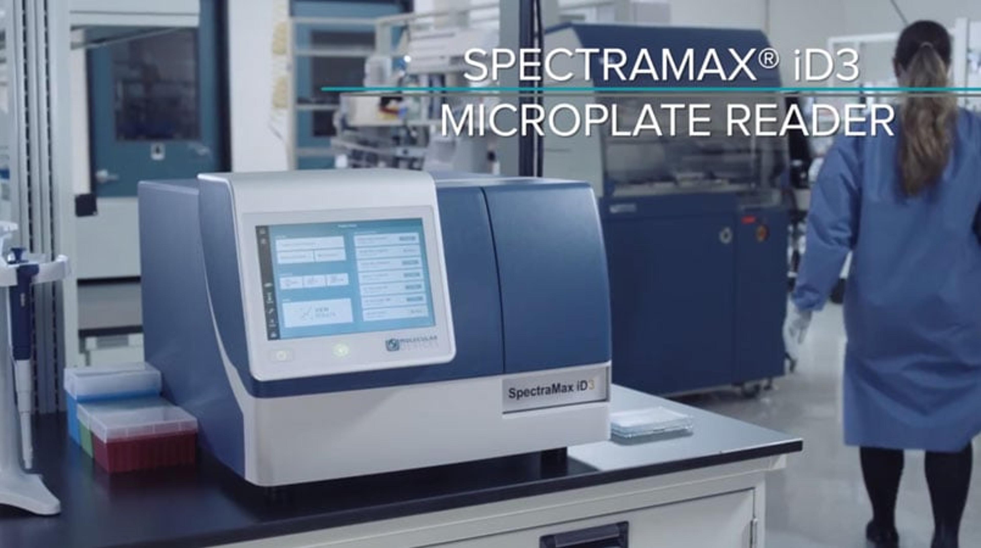
PDOs are generated from tumor biopsies or surgical procedures.
48
00:03:59.805 --> 00:04:04.351
They can serve as models to investigate different cancer mechanisms and, more
49
00:04:04.380 --> 00:04:09.015
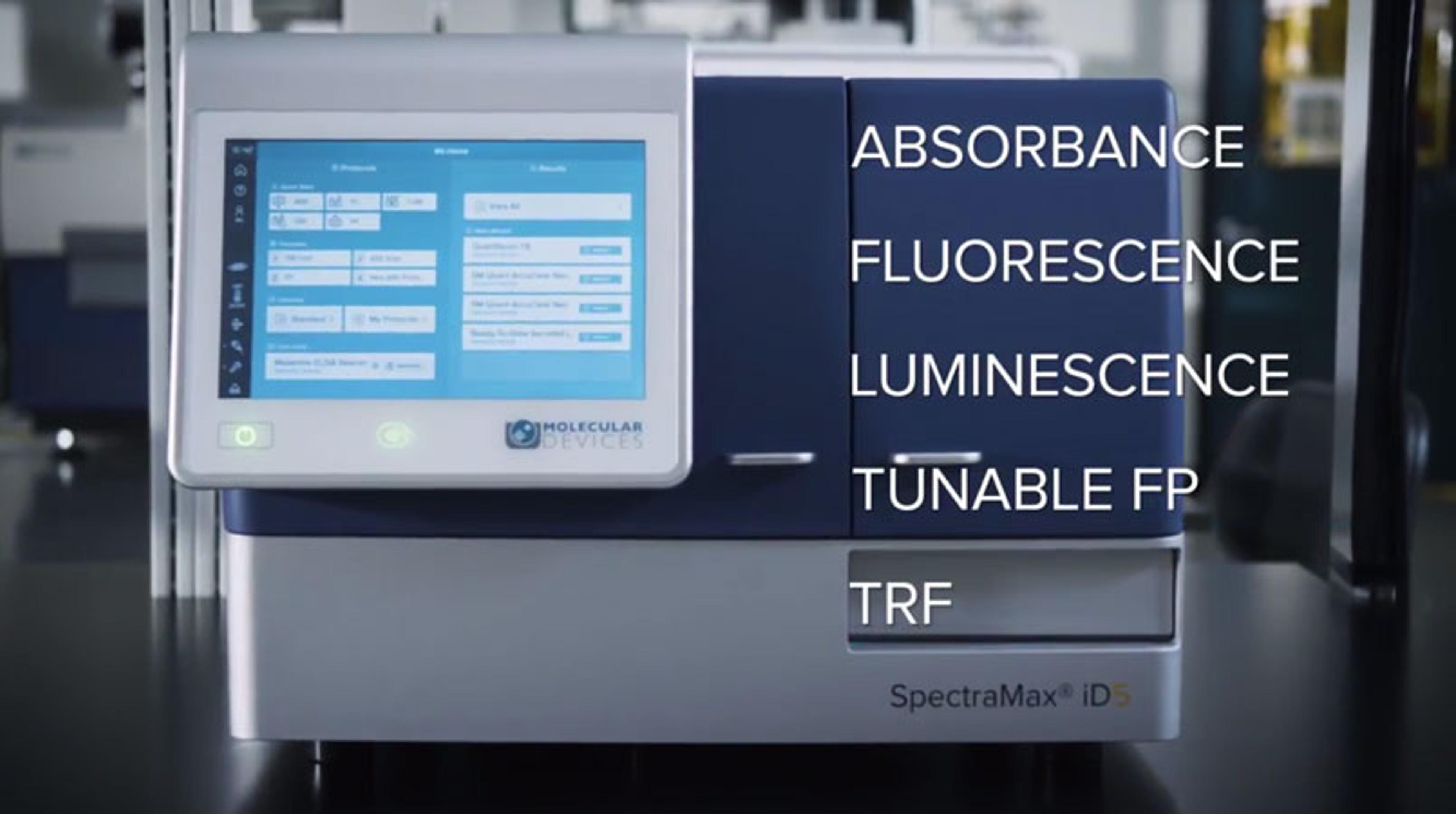
specifically, understand patient-specific drug responses.
50
00:04:09.810 --> 00:04:13.951
Because we know that different patients may react differently to different drugs.
51
00:04:14.505 --> 00:04:19.994
So instead of having the patient itself or themselves go through multiple
52
00:04:20.041 --> 00:04:25.500
reiterations of long drug testing, we can use PDOs to
53
00:04:25.591 --> 00:04:31.350
accurately predict patient responses to several different drugs and even
54
00:04:31.380 --> 00:04:34.170
investigate the effects of new novel drugs.
55
00:04:38.670 --> 00:04:43.080
Here's the general workflow for organoid culturing and screening.
56
00:04:43.140 --> 00:04:47.100
So the first step would be that 2D pre-culture.
57
00:04:47.160 --> 00:04:52.320
As stated, organoids are derived from either primary cells or induced pluripotent
58
00:04:52.410 --> 00:04:56.880
stem cells. And at this step, we are expanding these cells for the purpose of
59
00:04:56.940 --> 00:05:00.420
developing the 3D organoids here at step two.
60
00:05:01.591 --> 00:05:05.925
Typically, cells are pre-mixed with Matrigel, and then these droplets are placed
61
00:05:05.970 --> 00:05:10.109
into plates to form a 3D solid droplet dome.
62
00:05:11.040 --> 00:05:15.630
Media is then added, and to promote cell growth and differentiation into the
63
00:05:15.660 --> 00:05:16.800
specific tissue.
64
00:05:18.720 --> 00:05:23.970
Organoid culture is a bit of a process and may include several steps with different
65
00:05:24.031 --> 00:05:28.154
media. During this process, cell health should be monitored as well as
66
00:05:28.201 --> 00:05:32.355
characterized to ensure that they have the appropriate tissue structure and
67
00:05:32.400 --> 00:05:37.020
differentiation before moving forward with any further experiments.
68
00:05:42.660 --> 00:05:48.240
As you can see, it's really this step here, the organoid culture expanding, that
69
00:05:48.300 --> 00:05:53.370
can be a bit time-consuming. So to give you more of an idea,
70
00:05:54.690 --> 00:05:59.670
if we were to think about the manual process of sealing sufficient organoid
71
00:05:59.701 --> 00:06:04.635
material to perform a screen, it requires a lot of steps of passaging and
72
00:06:04.740 --> 00:06:10.545
reseeding. It would typically involve creating a lot of gel matrix domes in
73
00:06:10.591 --> 00:06:16.244
many wells from many plates. And this manual process can be time-consuming and
74
00:06:16.290 --> 00:06:21.510
requires highly trained staff. And even then, it can be prone to variability, which
75
00:06:21.540 --> 00:06:27.044
can then lead to inconsistencies in organoid size or morphology and
76
00:06:27.091 --> 00:06:32.401
ultimately mean that the process is challenging and quite a big
77
00:06:32.460 --> 00:06:33.151
investment.
78
00:06:36.750 --> 00:06:40.410
But worry not, we have a solution for you all.
79
00:06:40.454 --> 00:06:46.290
An alternative would be our 3D ready organoid expansion service.
80
00:06:46.350 --> 00:06:51.151
This is where we take your organoids and expand them in our proprietary BioReactor
81
00:06:51.210 --> 00:06:56.311
technology and provide them back to you in a frozen assay-ready format.
82
00:06:57.240 --> 00:07:01.651
So this technology can produce up to six million organoids in a batch.
83
00:07:01.740 --> 00:07:07.410
So let's say you're working with 96-well plates and you're using 100 to 200
84
00:07:07.470 --> 00:07:12.120
organoids per well. This allows you to work with hundreds of plates of data that
85
00:07:12.151 --> 00:07:14.760
all originate from the same batch.
86
00:07:15.750 --> 00:07:20.686
This means that you have a stock of high-quality off-the-shelf organoids.
87
00:07:21.240 --> 00:07:26.085
And when you're ready to begin your experiment, you can simply thaw, plate them
88
00:07:26.190 --> 00:07:29.790
out, and then test. Thaw, plate, and test.
89
00:07:34.651 --> 00:07:40.201
In summary, our 3D ready organoid expansion service not only provides you with
90
00:07:40.350 --> 00:07:45.390
large batches of standardized assay-ready organoids but also can save you a lot of
91
00:07:45.451 --> 00:07:51.180
time. If you were to do manual explored organoid expansion, it may take up to seven
92
00:07:51.270 --> 00:07:56.190
and eight weeks and ultimately result in batch-to-batch variation.
93
00:07:56.880 --> 00:08:00.780
Whereas with pre-expanded organoids, you are ready to start your treatment.
94
00:08:00.870 --> 00:08:06.451
All you have to do is thaw them out, and after about 48 hours, the organoids are
95
00:08:06.630 --> 00:08:11.730
ready to go. So from start to finish, this takes about a week and a half,
96
00:08:12.405 --> 00:08:16.350
which is a significant time savings to the project.
97
00:08:16.860 --> 00:08:20.520
Again, all you have to do is thaw, plate, and test.
98
00:08:22.530 --> 00:08:28.500
Speaking of test, that's a perfect segue to jump right into this data and the
99
00:08:28.561 --> 00:08:29.670
study that we did.
100
00:08:32.581 --> 00:08:37.290
The overall aim of this study was to demonstrate rapid characterization and
101
00:08:37.350 --> 00:08:42.030
assessment of candidate drug treatments in colorectal cancer organoids.
102
00:08:43.020 --> 00:08:47.100
Of course, big thank you to the team whose beautiful data I'm sharing with you
103
00:08:47.160 --> 00:08:47.550
today.
104
00:08:49.710 --> 00:08:55.350
So in this study, we used colorectal cancer organoids that we actually expanded
105
00:08:55.500 --> 00:08:59.790
using our handy-dandy 3D ready organoid expansion service.
106
00:09:00.585 --> 00:09:06.030
And just like the saying goes, we thawed the organoids, plated them in
107
00:09:06.240 --> 00:09:11.550
384-well microplates, and after 48 hours of recovery time,
108
00:09:11.940 --> 00:09:13.079
began our testing.
109
00:09:14.736 --> 00:09:20.240
After five days of selected anticancer compounds, organoid viability was
110
00:09:20.286 --> 00:09:25.716
assessed using both imaging with the ImageXpress in conjunction with a
111
00:09:25.777 --> 00:09:30.007
luminescent ATP cell viability assay on our
112
00:09:30.186 --> 00:09:33.021
SpectrumX.ID5 microplate reader.
113
00:09:36.036 --> 00:09:40.716
Here at Molecular Devices, we're in a unique position where we can really help you
114
00:09:40.836 --> 00:09:46.806
out in every step of this workflow, beginning with our 3D organoid expansion, where
115
00:09:46.836 --> 00:09:51.606
we can provide you with literally millions of standardized assay-ready organoids.
116
00:09:52.056 --> 00:09:56.345
And like the saying goes, again, you can thaw, plate, and then test them.
117
00:09:57.546 --> 00:10:02.166
And we can help with that monitoring and characterizing the organoids via our
118
00:10:02.226 --> 00:10:05.481
imaging system, the ImageXpress microconfocal.
119
00:10:07.176 --> 00:10:11.841
And lastly, we can also perform that plate reader assay using our
120
00:10:12.036 --> 00:10:17.257
SpectrumX.ID5, which is one of our instruments that we provide in our microplate
121
00:10:17.346 --> 00:10:22.626
portfolio. And you can also see that we can automate this system as well.
122
00:10:23.166 --> 00:10:28.896
So in this case, we actually have a team that can help you automate the adding of
123
00:10:28.956 --> 00:10:34.476
the reagent, the shaking, the incubation, as well as that automation of actually
124
00:10:34.507 --> 00:10:35.241
reading the plate.
125
00:10:36.576 --> 00:10:41.271
Again, we have a dedicated team here that can work with you to create a customized,
126
00:10:41.496 --> 00:10:44.316
automated workflow for whatever your needs are.
127
00:10:45.546 --> 00:10:47.406
So again, we're really here to help.
128
00:10:47.496 --> 00:10:51.141
In this particular workflow, we can really help you in every step of the way, and
129
00:10:51.156 --> 00:10:56.571
we're happy to learn and learn more about what your needs are and how we can help
130
00:10:56.736 --> 00:10:56.811
you.
131
00:11:01.626 --> 00:11:06.126
I'm going to highlight first the data that we got from our microplate reader.
132
00:11:08.616 --> 00:11:14.286
And so when people think of microplate readers, they usually think of simple assays
133
00:11:14.466 --> 00:11:19.596
like ECAs, Bradfords, ELISAs, and you're 100% right.
134
00:11:19.926 --> 00:11:25.536
You're not wrong. But I think what people tend to forget or even fail to recognize
135
00:11:25.777 --> 00:11:30.996
is just because these plate readers or these assays are relatively simple
136
00:11:31.086 --> 00:11:36.156
instruments, simple experiments, it doesn't make them any less effective,
137
00:11:36.876 --> 00:11:38.796
reliable, or impactful.
138
00:11:40.027 --> 00:11:44.856
Although the assays around the plate reader may not appear to be as complex as
139
00:11:44.916 --> 00:11:50.286
other experiments, the data you collect are just going to be just as reliable and
140
00:11:50.346 --> 00:11:52.836
robust, and most of the time, quicker.
141
00:11:53.286 --> 00:11:55.882
You're going to get that data quicker than other assays.
142
00:11:57.186 --> 00:12:02.106
Take ELISAs, for example. So ELISAs are very common assays, and they're very
143
00:12:02.226 --> 00:12:06.606
useful, and they're quick to do, especially if you can automate them.
144
00:12:07.806 --> 00:12:12.846
So not only are you getting good data, you're getting it in a relatively quick and
145
00:12:13.086 --> 00:12:14.016
easy manner.
146
00:12:15.216 --> 00:12:19.836
So don't discount or forget the power of a microplate reader.
147
00:12:23.046 --> 00:12:28.566
Here at MolDev, we have a large portfolio of both single-mode and multi-mode plate
148
00:12:28.626 --> 00:12:32.616
readers. Here are just a couple of our popular multi-mode readers.
149
00:12:33.546 --> 00:12:36.456
And we're proud to say that we're one of the trusted companies.
150
00:12:36.606 --> 00:12:40.446
One of our instruments here, the M5, is up in space.
151
00:12:40.686 --> 00:12:42.696
Two of them are actually up in space now.
152
00:12:43.236 --> 00:12:48.126
So you can trust that if our plate readers are up in space, that they'll do just as
153
00:12:48.157 --> 00:12:49.896
great down here on Earth.
154
00:12:55.326 --> 00:13:00.546
For this study, we used the SpectrumX.ID5, one of our multi-mode plate readers.
155
00:13:01.056 --> 00:13:07.040
And on the ID5, we performed Promega's CellTiter-Glo 3D Cell Viability
156
00:13:07.146 --> 00:13:12.966
Assay. You may have heard of this assay or maybe even used this kit on
157
00:13:12.996 --> 00:13:18.456
your 2D cultures, and this is basically the 3D version of the assay.
158
00:13:18.546 --> 00:13:23.210
If you're not familiar, the basic principle is that organoid cell death is
159
00:13:23.257 --> 00:13:28.657
indirectly assessed via a reduction of ATP levels.
160
00:13:28.716 --> 00:13:34.086
This is a luminescence assay, and the assay's luciferase reaction is depicted here
161
00:13:34.146 --> 00:13:38.856
on the right. It's a pretty basic add, mix, measure format.
162
00:13:39.246 --> 00:13:45.157
This results in cell lysis and generation of the luminescence signal proportional
163
00:13:45.171 --> 00:13:47.257
to the amount of ATP present.
164
00:13:48.786 --> 00:13:54.697
So in basic terms, more light, more cells, less light, less cells or dying cells.
165
00:13:56.736 --> 00:14:00.636
As I stated, most of the time, people don't usually think of a plate reader in
166
00:14:00.697 --> 00:14:03.846
association with 3D cultures like organoids.
167
00:14:04.236 --> 00:14:07.447
These are your precious patient-innovative samples.
168
00:14:07.536 --> 00:14:13.401
But this is a perfect example of how you can use your complex samples, such as your
169
00:14:13.507 --> 00:14:19.416
organoids, in conjunction with a plate reader to get quick and reliable data,
170
00:14:20.017 --> 00:14:23.526
which can ultimately save you a lot of time and money.
171
00:14:26.286 --> 00:14:31.896
Speaking of saving time, the CellTiter-Glo protocol is actually
172
00:14:32.046 --> 00:14:36.996
one of the over 140 pre-uploaded protocols in SoftMax
173
00:14:37.056 --> 00:14:42.411
Pro. SoftMax Pro is our data acquisition and analysis software
174
00:14:43.026 --> 00:14:48.036
and is the most published microplate reader control and microplate data analysis
175
00:14:48.096 --> 00:14:53.736
software package. One of my favorite things about the software is how user-friendly
176
00:14:53.826 --> 00:14:59.436
it is. Here's a little snapshot of our protocol manager, which houses the different
177
00:14:59.586 --> 00:15:03.231
categories of all of our pre-uploaded protocols that we have.
178
00:15:04.701 --> 00:15:09.801
I actually used SoftMax Pro when I was a post-doc, and even without any formal
179
00:15:09.846 --> 00:15:15.007
training on the software, I found it really easy to do my experiments and do some
180
00:15:15.066 --> 00:15:18.757
in-depth data analysis immediately after the plate was ran.
181
00:15:19.746 --> 00:15:24.322
So we really try to make it as easy as possible so that all you have to do is put
182
00:15:24.336 --> 00:15:27.757
the plate in and you're set to go.
183
00:15:29.436 --> 00:15:32.496
Now on to the good stuff, the data.
184
00:15:34.206 --> 00:15:38.960
The main aim of the study was to demonstrate a rapid quantitative analysis of drug
185
00:15:39.007 --> 00:15:43.955
responses in patient-derived colorectal cancer, or CRC, organoids.
186
00:15:45.155 --> 00:15:51.036
Organoids were seeded into 384-well microplates at 250 organoids
187
00:15:51.157 --> 00:15:56.451
per well and treated with three anticancer compounds,
188
00:15:56.856 --> 00:16:01.386
including cisplatin, doxorubicin, and remdesin for five days.
189
00:16:02.166 --> 00:16:07.056
This was performed in quadruplicate wells, each in a four-fold dilution series.
190
00:16:09.246 --> 00:16:14.977
Again, we used Promega's CellTiter-Glo 3D Cell Viability Assay, where an
191
00:16:15.036 --> 00:16:20.227
ATP production, and subsequently luminescent signal, is indicative of cell
192
00:16:20.376 --> 00:16:21.096
viability.
193
00:16:22.686 --> 00:16:27.501
Using the pre-configured protocol in SoftMax Pro, we were able to get results in
194
00:16:27.546 --> 00:16:29.796
this graph almost instantaneously.
195
00:16:31.341 --> 00:16:36.846
The x-axis is showing the concentration of the drug, with the y-axis depicting the
196
00:16:36.936 --> 00:16:39.336
average relative luminescence units.
197
00:16:40.776 --> 00:16:45.126
And what I hope you can appreciate from this graph, from this data, is not only the
198
00:16:45.157 --> 00:16:50.767
effects of the different drugs on the CRC organoids, but also the dose at which it
199
00:16:50.826 --> 00:16:56.572
is the most effective. So even from a simple add-mix-read format, you're able to
200
00:16:56.586 --> 00:17:02.166
get quality drug response information, including the magnitude of effects, as well
201
00:17:02.197 --> 00:17:04.477
as the dose-dependent effects of the drugs.
202
00:17:05.646 --> 00:17:11.001
And furthermore, remember that these are patient-derived CRC organoids, organoids
203
00:17:11.017 --> 00:17:14.076
coming directly from the patient themselves.
204
00:17:14.106 --> 00:17:19.236
Thus, even at a plate-based experiment, it can be translated as personalized
205
00:17:19.267 --> 00:17:19.806
medicine.
206
00:17:21.517 --> 00:17:23.856
And finally, this is a quick assay.
207
00:17:24.276 --> 00:17:29.916
Reagent handling, assay detection, and analysis was all done in about 30 minutes.
208
00:17:30.531 --> 00:17:34.026
And mind you, 25 minutes of that time was incubation time.
209
00:17:34.596 --> 00:17:39.456
So really, based off your experimental design, in about five minutes of work, you
210
00:17:39.486 --> 00:17:45.006
can get a walkaway solution for assessing drug effects in patient-derived
211
00:17:45.126 --> 00:17:45.741
organoids.
212
00:17:48.246 --> 00:17:53.136
I hope I convinced you or remind you of the power of the microplate reader and the
213
00:17:53.166 --> 00:17:56.721
wealth of data it can give you in a simple and rapid manner.
214
00:17:57.697 --> 00:18:01.326
But we also want to show you the imaging side of the study, where we did
215
00:18:01.447 --> 00:18:06.456
confirmation studies of the organoid size and morphology using the ImageXpress.
216
00:18:07.506 --> 00:18:11.346
So from here, I'll hand it to my colleague, Dr. Angeline Lim.
217
00:18:15.318 --> 00:18:19.578
Thanks, Crystal. And so while Crystal earlier showed an example of a plate
218
00:18:19.608 --> 00:18:25.008
reader-based endpoint assay, there are other relatively simple data that you can
219
00:18:25.098 --> 00:18:28.488
also acquire from experiment before you get to that point.
220
00:18:28.548 --> 00:18:33.198
And so I'm going to focus on this part of the workflow where this is the time where
221
00:18:33.228 --> 00:18:37.668
you can actually collect more data and glean some useful information from the
222
00:18:37.698 --> 00:18:42.543
experiment. And so with an imager, you can monitor the growth of the organoid in
223
00:18:42.618 --> 00:18:45.108
culture, basically monitor compound effects.
224
00:18:45.573 --> 00:18:49.159
An example of what you can glean from a combination of imaging and endpoint
225
00:18:49.218 --> 00:18:54.034
viability assay is the ability to tease apart whether a compound is cytostatic or
226
00:18:54.168 --> 00:18:57.138
cytotoxic, or a combination of both.
227
00:18:57.198 --> 00:19:01.008
And to tell if a compound is inhibiting your organoid growth, you can first
228
00:19:01.278 --> 00:19:05.478
observe, but of course, as a scientist, we like to quantitate this observation by
229
00:19:05.538 --> 00:19:07.909
measuring the size of organoids from the images.
230
00:19:10.938 --> 00:19:13.578
And how would one typically go about doing this?
231
00:19:13.998 --> 00:19:18.738
And I would say using the more conventional approach with image analysis,
232
00:19:20.208 --> 00:19:23.748
you would want to set up an image analysis pipeline.
233
00:19:23.762 --> 00:19:27.964
And one of the most important steps in the pipeline is known as segmentation, where
234
00:19:27.978 --> 00:19:30.918
the structure of interest is identified.
235
00:19:30.948 --> 00:19:35.418
And so this more classical approach tends to be very rule-based.
236
00:19:35.478 --> 00:19:39.528
And over here, I'll illustrate what I mean with this example over here on the
237
00:19:39.558 --> 00:19:44.868
screen. So on the left, this is the input image, where there you can see it.
238
00:19:44.899 --> 00:19:50.343
It's not a pretty image, but this is a great example because here we are actually
239
00:19:50.358 --> 00:19:54.348
looking at iPSC colonies, and there's a little bit of debris at the upper left-hand
240
00:19:54.409 --> 00:20:00.153
corner. And what I really want to get out of this set of image analysis is right at
241
00:20:00.168 --> 00:20:03.589
the end on the right side, which is I want to create a mask that identifies my
242
00:20:03.603 --> 00:20:06.573
structure of interest, which is I want to measure the area of these stem cell
243
00:20:06.589 --> 00:20:11.284
colonies. And to get there, I first have to apply a couple of image processing
244
00:20:11.328 --> 00:20:15.978
tools. So for example, I had a Gaussian blur. I set the parameters for it.
245
00:20:16.068 --> 00:20:20.478
I did a math operation with a gradient filter, morphological filter, open size
246
00:20:20.508 --> 00:20:24.318
filter, so on and so forth, so that I can finally get that image.
247
00:20:24.918 --> 00:20:27.528
However, this does not always work,
248
00:20:29.058 --> 00:20:32.778
because once we look at an image from even from within this experiment, you would
249
00:20:32.868 --> 00:20:38.358
see that this pipeline picked up not just the colony, but also some debris on the
250
00:20:38.418 --> 00:20:43.878
lower left side, and also it picked up this sort of shading artifact on the top
251
00:20:43.938 --> 00:20:48.798
right side, which is not what I want. And so in other words, oops.
252
00:20:48.858 --> 00:20:51.843
In other words, there are limitations to the conventional
253
00:20:53.058 --> 00:20:56.163
segmentation approach, because it's very rule-based, it's very manual.
254
00:20:56.238 --> 00:20:59.223
You have to be sitting there trying to figure out what's the best parameter that
255
00:20:59.238 --> 00:21:01.159
will work for the entire experiment.
256
00:21:01.248 --> 00:21:05.223
The algorithms or analysis pipeline that you optimize for some image or some field
257
00:21:05.268 --> 00:21:08.718
of view may not work for the entire experiment, as we saw over here.
258
00:21:08.733 --> 00:21:11.298
And the rules could vary between experiments.
259
00:21:11.358 --> 00:21:15.589
And sometimes you would have set up two different analysis protocol just for this
260
00:21:15.618 --> 00:21:19.188
experiment, and really that's not the ideal way of doing it.
261
00:21:19.488 --> 00:21:23.823
And so, in other words, you can see that there's limited accuracy and usability,
262
00:21:24.409 --> 00:21:29.598
and I think quite often it tends to lead to user frustration, and it's basically an
263
00:21:29.628 --> 00:21:31.518
inefficient way of doing this.
264
00:21:32.718 --> 00:21:36.228
And so here is where I found that AI can be a very powerful approach.
265
00:21:36.858 --> 00:21:41.958
At Molecular Devices, we have the Encarta image analysis software, and that plugin
266
00:21:41.988 --> 00:21:46.818
or that module is we refer to as SNAP, which stands for segmentation is not a
267
00:21:46.848 --> 00:21:51.558
problem. And so here is a little workflow to illustrate what you would do starting
268
00:21:51.589 --> 00:21:55.488
from the image set. You would annotate images and then create your training set of
269
00:21:55.548 --> 00:21:58.998
data, and then you would train it. Now, all of this may sound very intimidating to
270
00:21:59.028 --> 00:22:01.758
someone that doesn't, you know, not an AI expert.
271
00:22:01.818 --> 00:22:07.113
So what we've done is we have made it very user-friendly, such that you don't have
272
00:22:07.159 --> 00:22:11.238
to be an expert to run it. And I'll just illustrate this by showing you how the
273
00:22:11.268 --> 00:22:13.563
software looks like and what you would do as a user.
274
00:22:14.388 --> 00:22:18.858
So first thing you would do is, of course, open the software and get into the SNAP
275
00:22:19.308 --> 00:22:21.708
interface, and you would load your image.
276
00:22:22.068 --> 00:22:25.128
So here is an example of the image I've loaded.
277
00:22:25.428 --> 00:22:30.978
You're looking at spheroids that were grown in these multi-cavity plates.
278
00:22:31.128 --> 00:22:36.018
And then using the left side of the interface, there are sort of some tools
279
00:22:36.078 --> 00:22:37.638
available for you to do annotation.
280
00:22:37.818 --> 00:22:43.159
And by annotation, it simply refers to, as a user, you want to sort of
281
00:22:43.278 --> 00:22:47.508
identify what are the structures that you're interested in versus what is
282
00:22:47.568 --> 00:22:52.638
considered background. And so in this example over here, anything that is in green,
283
00:22:53.178 --> 00:22:55.923
I'm trying to tell the software that, hey, this is what I really want to measure,
284
00:22:56.089 --> 00:23:00.048
and then I try to give example of what I don't want to measure.
285
00:23:00.108 --> 00:23:02.808
So that's the stuff that you see shaded in blue.
286
00:23:03.272 --> 00:23:06.964
And you would repeat this and gather a couple of these, well, not a couple, it
287
00:23:06.978 --> 00:23:12.078
depends. You'll gather some amount of these training images, save it
288
00:23:13.008 --> 00:23:17.958
as a training set, and then you will hit on the software, you hit the software
289
00:23:18.018 --> 00:23:21.977
train. Okay? And this is when sort of the AI magic happens.
290
00:23:22.758 --> 00:23:28.698
The software would just do its training using a neural network.
291
00:23:28.758 --> 00:23:32.418
And all of this happens in the background, so that what you do is you hit train,
292
00:23:32.448 --> 00:23:34.608
you basically walk away and go do other things.
293
00:23:36.288 --> 00:23:39.978
At the end of the training, what the software would do is it will apply that train
294
00:23:40.038 --> 00:23:44.089
model on the current set of images, and then you can evaluate whether it looks good
295
00:23:44.149 --> 00:23:47.508
or not. And in this case, you can see it's not great because it's picking out all
296
00:23:47.628 --> 00:23:48.198
these other
297
00:23:49.548 --> 00:23:53.028
sort of areas that's around the micro cavities.
298
00:23:53.508 --> 00:23:56.988
And if this is the case, what you can do is you would repeat steps one to three,
299
00:23:57.468 --> 00:24:01.488
add in a couple more training images, and then retrain as needed, such that
300
00:24:01.758 --> 00:24:04.878
eventually you would get to something that looks a lot better, and then you would
301
00:24:04.968 --> 00:24:07.682
save this model and use that in your image analysis pipeline.
302
00:24:12.048 --> 00:24:17.163
And so, what are the benefits of using such an approach for image analysis?
303
00:24:17.628 --> 00:24:20.988
And so I've illustrated the workflow, and it's pretty straightforward and easy to
304
00:24:21.078 --> 00:24:25.473
use, I would say. But other advantages that I want to highlight here is that using
305
00:24:25.518 --> 00:24:29.147
this approach, your image analysis pipeline can be very robust.
306
00:24:29.208 --> 00:24:33.498
So as example, on the right side of the screen, you can see over here these are CRC
307
00:24:33.528 --> 00:24:39.137
organoids that were grown in a 3D4 plate and do an image at pretty low mag, do a 4X
308
00:24:39.198 --> 00:24:44.868
objective. And what I myself was surprised when I saw this was that when I ran the
309
00:24:44.928 --> 00:24:49.998
analysis, I found a bunch of organoids that were picked up in the top left of the
310
00:24:50.073 --> 00:24:54.363
image. But when I zoom in and look closer, I realized, hey, there are images there
311
00:24:54.409 --> 00:24:58.458
that I didn't see by eye at a glance, but the software or the model picked it up.
312
00:25:00.798 --> 00:25:04.308
And another area where I think it's really robust, and this was also a huge
313
00:25:04.339 --> 00:25:08.613
surprise to me, was that sometimes when you culture your organoids or when you seed
314
00:25:08.718 --> 00:25:14.418
them, having bubbles either in the media or on your major gel, it could happen.
315
00:25:14.448 --> 00:25:20.298
And when that happens, usually you would think it's difficult to image or analyze
316
00:25:20.358 --> 00:25:23.958
what's under the bubbles. But in this case, I was surprised that the model actually
317
00:25:24.018 --> 00:25:26.089
picked up an organoid that was under the bubble, too.
318
00:25:26.118 --> 00:25:30.198
And so if you look at the inset, there's a zoom-in close-up image of that bubble,
319
00:25:30.258 --> 00:25:34.399
and you can see that it did pick up one object there. All right.
320
00:25:35.284 --> 00:25:38.988
So besides being robust, the other thing to note is that if you have a well-trained
321
00:25:39.048 --> 00:25:43.368
model, that model can be used over and over without having to retrain or do
322
00:25:43.458 --> 00:25:47.748
tweaking or changes. So here's an example where one model was applied to just the
323
00:25:47.779 --> 00:25:52.339
entire set, not just the plate, but also to the images that were acquired over days
324
00:25:52.368 --> 00:25:58.353
in culture. So these are, again, CRC organoids, and from left to right
325
00:25:58.399 --> 00:26:03.514
is like day one all the way to the increasing number of
326
00:26:03.589 --> 00:26:08.149
days. And the color, it's overlay with sort of a colored...
327
00:26:09.348 --> 00:26:13.848
It has a color overlay to identify or to show what the model has identified as
328
00:26:13.938 --> 00:26:16.878
structures to measure in the analysis pipeline.
329
00:26:19.339 --> 00:26:23.328
All right. And another point to note, too, is because you don't have to set all the
330
00:26:23.389 --> 00:26:27.618
rules, you just show the software what you want in your training set.
331
00:26:27.678 --> 00:26:31.158
It allows for you to segment really complex structures, and I'm going to show some
332
00:26:31.188 --> 00:26:36.708
example here. Here you're looking at human pancreatic organoids that were grown in
333
00:26:36.738 --> 00:26:40.548
Grid3D plate from Some BioSciences, and so basically there's a lot of little micro
334
00:26:40.639 --> 00:26:42.438
cavities in each well of this plate.
335
00:26:43.248 --> 00:26:47.149
And so the first thing we did is we created a model to identify the cavities.
336
00:26:48.408 --> 00:26:51.318
You may not have to do this if that's not what you want to measure.
337
00:26:52.173 --> 00:26:56.748
Next, we have a model that then identified the organoid.
338
00:26:57.393 --> 00:27:01.669
And then we were also interested in sort of quantifying sort of the hollow lumen or
339
00:27:01.698 --> 00:27:05.658
the more cystic part of these organoids, and so we also created a model to help
340
00:27:05.688 --> 00:27:09.333
measure that. And so that's what you see in blue. All right.
341
00:27:09.348 --> 00:27:14.508
And then I also think that with deep learning, it's really useful to also analyze
342
00:27:14.538 --> 00:27:17.823
things that may look simple, but when you're trying to set up the analysis, it's
343
00:27:17.839 --> 00:27:23.574
really hard, it's really tough. Bright field images, non-fluorescent Our label-free
344
00:27:23.634 --> 00:27:25.554
images is, I think, a prime example.
345
00:27:26.154 --> 00:27:29.574
So in this case, we have a model that will identify iPSC colonies.
346
00:27:30.594 --> 00:27:35.049
We have also trained models to identify differentiated versus non-differentiated
347
00:27:35.094 --> 00:27:40.840
cells, which we think is really useful for researchers that are doing iPSC and
348
00:27:41.124 --> 00:27:42.084
growing all iPSCs.
349
00:27:43.734 --> 00:27:48.309
And then, another benefit that I think is great when you use this deep
350
00:27:48.355 --> 00:27:52.029
learning-based approach in our software is that you don't need to be an expert in
351
00:27:52.074 --> 00:27:56.124
image analysis. You don't have to know exactly which algorithm to use or which
352
00:27:56.154 --> 00:28:00.370
specific tool to use, whether you should do a Gaussian blur or whether you should
353
00:28:00.715 --> 00:28:05.754
do other kind of processing to your images so that you get a good segmentation.
354
00:28:05.814 --> 00:28:11.620
Right? And usually, the way I see it, or my advice is if you can see it, you can
355
00:28:11.665 --> 00:28:14.259
train it, and you can therefore measure it.
356
00:28:16.284 --> 00:28:19.134
And so now back to the data that Crystal shared earlier.
357
00:28:19.254 --> 00:28:24.114
So here's an example of when we do the monitoring, and so we image the plate over
358
00:28:24.204 --> 00:28:27.564
time, over days in culture, and we did that pre-treatment and post-treatment.
359
00:28:28.090 --> 00:28:31.344
And so here you can see the compound effects on CRC growth.
360
00:28:31.644 --> 00:28:34.194
I've shown just two examples of the two compounds here.
361
00:28:34.824 --> 00:28:39.294
Top row is the DMSO control, and we can measure that at the end of the experiment,
362
00:28:39.355 --> 00:28:44.544
the growth of the organoid is about two and a half or it's a fourfold increase in
363
00:28:44.605 --> 00:28:50.544
size. 5-Fluorouracil did show changes in size, but morphologically, you can tell
364
00:28:50.605 --> 00:28:54.204
that the structure is a little bit different. It looks actually quite cystic.
365
00:28:54.909 --> 00:28:59.783
And the bottom row is doxorubicin, where you can see that post-treatment, nothing
366
00:28:59.844 --> 00:29:05.004
grows. It's definitely not growing, and we also saw earlier that it's also
367
00:29:05.514 --> 00:29:08.304
cytotoxic. Right? There was very low viability.
368
00:29:09.984 --> 00:29:15.564
And so here is sort of a summary of all the compounds that I've tested.
369
00:29:17.605 --> 00:29:21.054
And here is a video playing that just shows the
370
00:29:22.314 --> 00:29:23.904
growth of the organoids over time.
371
00:29:24.024 --> 00:29:28.239
I pointed out too that this is sort of a histogram where on the y-axis is area, on
372
00:29:28.254 --> 00:29:32.245
the x is days in culture. So if we just focus on the middle panel, the middle
373
00:29:32.694 --> 00:29:38.094
chart, it's showing that over time, each dot represents each single organoid.
374
00:29:38.544 --> 00:29:41.605
So all the organoids, eventually they do get bigger, so you can see the trend
375
00:29:41.634 --> 00:29:46.584
towards a larger area. Whereas with doxorubicin, you can see obviously, they all
376
00:29:46.644 --> 00:29:52.105
sort of get arrested. Romidepsin is another one that we saw, too.
377
00:29:52.314 --> 00:29:56.725
What's interesting, too, is that there are times when we see, and actually quite
378
00:29:56.754 --> 00:29:58.764
frequently, we see that drugs would have
379
00:30:00.294 --> 00:30:05.605
impacts or would affect growth. So you can see there's no change in the organoid
380
00:30:05.694 --> 00:30:10.600
size, but we don't see toxicity with our viability endpoint assay.
381
00:30:10.629 --> 00:30:14.379
And so it suggests all different mechanisms of action, too, which I think is
382
00:30:14.424 --> 00:30:14.874
interesting
383
00:30:17.034 --> 00:30:20.814
information to have as well when you're doing this kind of assays.
384
00:30:20.874 --> 00:30:26.394
And so just to summarize it all, we believe that organoid technology holds
385
00:30:26.634 --> 00:30:31.194
significant promise in transforming the drug discovery landscape and definitely in
386
00:30:31.254 --> 00:30:32.995
advancing personalized medicine.
387
00:30:33.564 --> 00:30:35.993
And at Molecular Devices, we are
388
00:30:37.523 --> 00:30:43.254
trying, or we would like to help you on that journey by really trying to identify
389
00:30:43.284 --> 00:30:46.794
the bottlenecks and coming up with solutions to help you.
390
00:30:47.350 --> 00:30:52.074
And one of the gaps that we see is that it's difficult for most people to scale up
391
00:30:52.165 --> 00:30:56.484
their organoids to a good enough scale or to a large
392
00:30:57.774 --> 00:31:01.614
enough scale with quality and quantity that they are ready to do screening.
393
00:31:01.644 --> 00:31:05.769
And so to that end, I want to point out that we do have a service now.
394
00:31:06.264 --> 00:31:11.965
It's a bioreactor-based system that we can use in-house to scale up your
395
00:31:12.054 --> 00:31:15.745
specific organoid of interest. And so at the end of the day, what we send back to
396
00:31:15.804 --> 00:31:19.344
you are these cryopreserved, cryo-frozen vials of organoids.
397
00:31:19.465 --> 00:31:22.944
So what you usually would have to do is just thaw them out, and as Crystal
398
00:31:22.975 --> 00:31:27.355
mentioned, it's ready to run your assay within 48 hours. All right.
399
00:31:28.764 --> 00:31:33.954
The last point here is with microplate reader-based viability assay, in combination
400
00:31:34.014 --> 00:31:38.725
with label-free imaging, and then again, using the AI-assisted image analysis
401
00:31:38.784 --> 00:31:43.584
software, it's a very powerful combination and a powerful and efficient combination
402
00:31:43.614 --> 00:31:47.904
which can serve as a preliminary approach to really speed up the identification of
403
00:31:47.965 --> 00:31:50.364
potential hits in your screen.
404
00:31:51.864 --> 00:31:56.109
Yeah, and you could derive things or get ideas on mechanism of actions or really
405
00:31:56.154 --> 00:32:00.294
see what the compounds are doing with this combination approach.
406
00:32:01.524 --> 00:32:06.804
And with that, I've come to the end of this webinar,
407
00:32:07.044 --> 00:32:11.694
and we are open to questions now from the audience.
Related products
Request Quote for All Products
SoftMax® Pro GxP Software
Molecular Devices®Meet FDA guidelines in GMP/GLP labs with complete validation tools
SoftMax® Pro Microplate Data Acquisition & Analysis Software
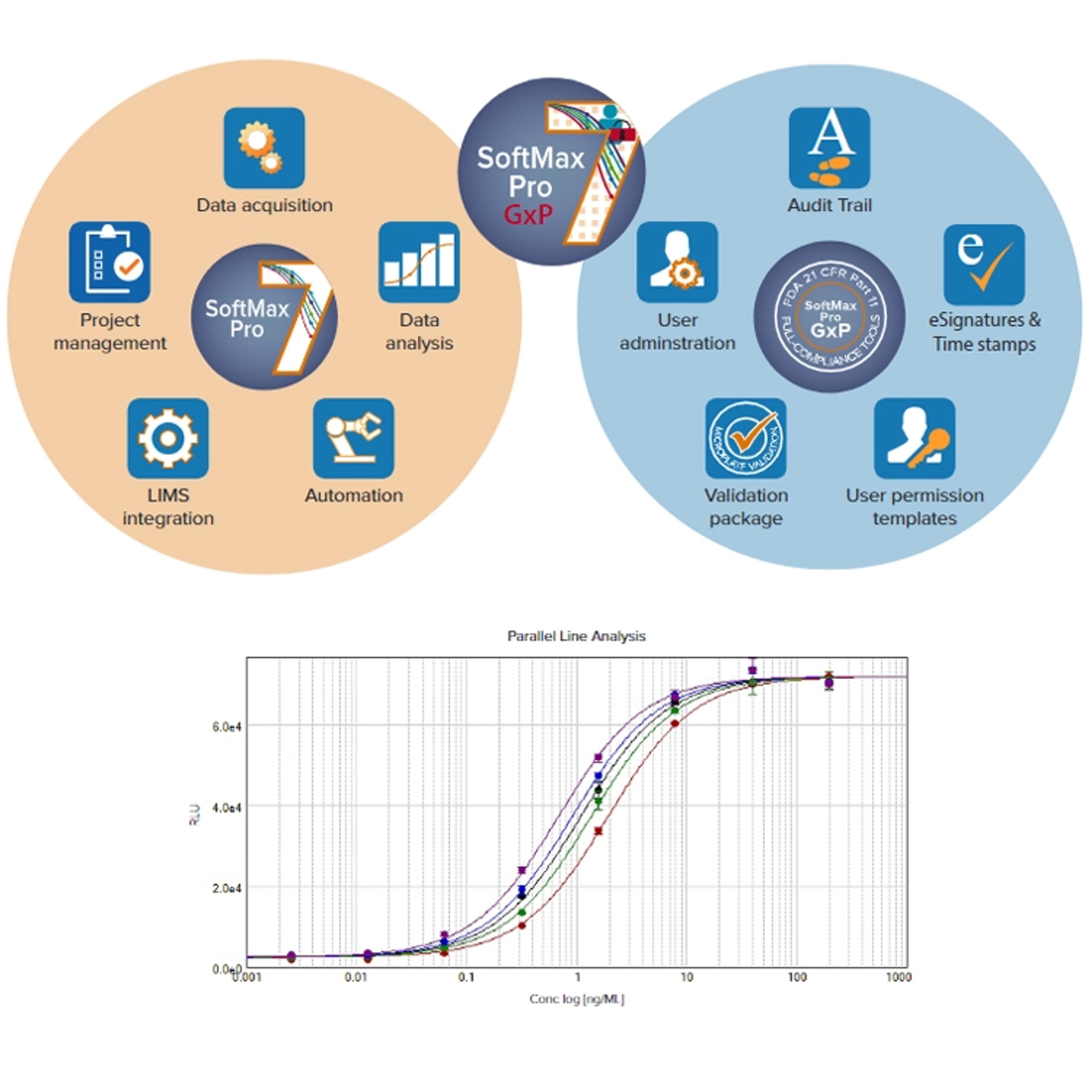
Molecular Devices®SoftMax ® Pro Software is designed to provide the simplicity, flexibility and power required for advanced data analysis. It provides ready-to-run protocols, analysis algorithms, and 21 different curve fit options. Every step has been optimized for data acquired from a Molecular Devices microplate reader or data imported from another source to simplify analysis and reporting. FDA 21 CFR Part 11 compliance tools are available for regulated laboratories providing end-to-end chain of custody.